In previous posts of this series I have shown that a Resnet56V2 with AdamW can converge to acceptable values of the validation accuracy for the CIFAR10 dataset – within less than 26 epochs. An optimal schedule of the learning rate [LR] and optimal values for the weight decay parameter [WD] were required. My network – a variation of the ResNetV2-structure of R. Atienza [1] – had 1.67 million trainable parameters, only. Therefore, I was satisfied with reaching a validation accuracy threshold of val_acc = 0.92 for CIFAR10. However, a convergence before or at epoch 20 could not be reproduced systematically, yet. In addition: For significantly longer runs over more than 40 up to 60 epochs) better accuracy values 0.924 < val_acc < 0.931 were achievable (see previous posts). Below I will show what kind of changes to the ResNet reproducibly enable a convergence for the validation accuracy threshold before or at epoch 20 – and give values above 0.924 for 84% of the training run ahead of epoch 25 – without changing the number of Conv2D-layers. One of the tricks is to change the kernel-size of the convolutional shortcut layer in the first Residual Unit of each Residual Stack.
Links to previous posts:
- AdamW for a ResNet56v2 – II – linear LR-schedules, Adam, L2-regularization, weight decay and a reduction of training epochs
- AdamW for a ResNet56v2 – III – excursion: weight decay vs. L2 regularization in Adam and AdamW ,
- AdamW for a ResNet56v2 – IV – better accuracy and shorter training by pure weight decay and large scale fluctuations of the validation loss ,
- AdamW for a ResNet56v2 – V – weight decay and cosine shaped schedule of the learning rate
Changes and Setup
Regarding the structure of my ResNetV2 network used in this investigation of super-convergence preconditions I refer to [1], [2] and [3]. A sequence of m Main Residual Stacks [RSs] consist of n Residual Units [RUs]. Each RU comprises 3 regular Conv2D + 1 Conv2D-layer used as a shortcut layer at the very first RU of each RS. See the illustrations in [3]. The layer structure followed closely a recipe published by R. Atienza in [1].
Where might such a ResNet have weak properties? There are multiple points which one might think of. For this post I introduced 3 changes, which lead to more trainable parameters, but do not change the number of Convolutional Layers of the Resnet.
Change 1 – no pooling ahead of the fully connected part: The first critical point is something that we also find in [4]. Ahead of the final fully connected [fc] network with a softmax-activation we find some pooling-layer in the standard recipe for the transition from the ResNet to the analyzing fc-structure. Looking at the Github code of Atienza [2] reveals that he, too, applies a pooling layer ahead of flattening. For 3 Residual Stacks [RS] the last Conv2Ds of stack RS=3 deal with maps of dimension [8×8]. Atienza applies the following:
    # x = Output from last adding layer of RS 3 for maps with size [8x8]
    x = AveragePooling2D(pool_size=8)(x)
    y = Flatten()(x)
    outputs = Dense(num_classes,
                    activation='softmax',
                    kernel_initializer='he_normal')(y)
Do we need this? Of course, pooling saves some trainable parameters. However, for the runs below I omitted the AveragePooling2D layer. This gives our analyzing fc-network more ways to adapt.
Change 2 – (3×3)-kernel for the Shortcut Conv2D layers: There is only one gateway in all Residual Units which decides upon how strongly the original input mixes with the processed output of the RU’s layer sequence. This is at the convolutional shortcut layer of the very first RU of each Residual Stack [RS]. There we must apply strides=2 to account for dimension reduction. In standard ResNet-recipes a kernel-size of (1×1) is used. This can be disputed. For my tests below I used a (3×3)-kernel for these specific Conv2D Shortcut layers. Note that for 3 RS we just have two such layers.
Change 3 – Batch Normalization and Activation for the Shortcut Conv2D layers: In [5] we read at the section for implementation details: “For the bottleneck ResNets, when reducing the feature map size we use projection shortcuts [1] for increasing dimensions, and when preactivation is used, these projection shortcuts are also with pre-activation.” Bold face emphasis done by me.
However, looking at the code in [2] we see that Atienza explicitly turned off pre-activation. I changed this in some special runs below (see table 2). Because preliminary tests showed that Batch Normalization [BN] should be added, too, I did most test runs for all combined changes (1 to 3) with BN active for the shortcut layers.
Other general properties of my ResNet are:
- Numbers of RS and RUs: As in previous runs of the post series I used 3 Residual Stacks, each with 6 Residual Units with the V2-layer structure described in [3] and [4] .
- Increase of the number of trainable parameters: The first two measures raised the total number of trainable parameters to 2.17 million, i.e. roughly by a factor of 1.3.
- Statistically selected data for the validation set: The validation data set was statistically rebuild for every run – but in a stratified way with the help of SkLearn’s funtion train_test_split().
- Batch shuffling: Batches during training were shuffled. The chosen Batch Size [BS] was BS=64.
- HeloNormal as weight initializer: Weights were initialized by the HeloNormal initializer.
- AdamW as optimizer: AdamW with decoupled weight-decay was used in all runs – L2-regularization was explicitly and totally deactivated. The weight decay parameter (for decoupled weight decay) is called WD below.
Balanced cosine LR-schedules
From experiences with previous runs (see the previous posts) we know two things: 1) A value of LR=0.0008 is somewhat optimal on average. 2) Fast convergence can be reached by a cosine decline after a plateau phase. Therefore I did not change the basic scheduling for short runs structurally: We start with a linear rise, stay on a plateau and then move along a cosine shaped LR-decay. However, we need to balance the decline. By some experiments I found that the two following variants were helpful:
Illustration 1: LR-schedule Type I – low plateau, later and shorter cosine decay
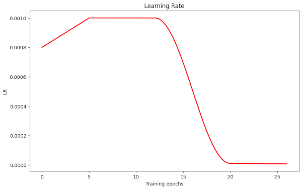
The plateau has a LR-value of LR=0.001. We start a decay at epoch 12 to reduce the LR to optimal values of 0.0008 at around epoch 15.
Illustration 2: LR-schedule Type II – higher plateau, earlier and longer cosine decay
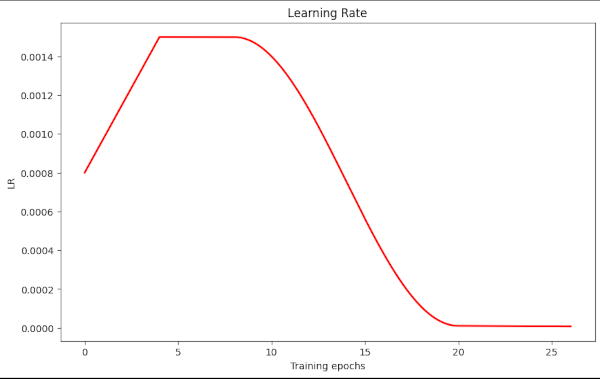
In this case we go up to LR=0.0015, the plateau ranges from epoch 4 to epoch 8, only. We start an early decay to reduce the LR to optimal values of 0.0008 already at epoch 15.
Results for combined changes 1 and 2
As in the previous posts I summarize the results of performed example runs in a table 1. See there for an explanation of the columns. Regarding the LR schedule: “lin” means a linear change in LR, “cos” a cosine shaped decline in LR. Please, do not care about the strange numbering of the runs. “Mixed prec.” characterizes runs done with Keras “mixed precision” (16-Bit/32-Bit) to save energy consumption of the graphics card.
You may have to look at the table on a PC or laptop to see all columns.
Table 1 – runs up to 25 epochs – with changes 1 and 2 in place
| # | epoch | acc_val | acc | epo best | val acc best | final loss | final val loss | shift | l2 | λ | α max | LR reduction phases | Remark |
| 58 | 20 | 0.92380 | 0.9613 | 25 | 0.92580 | 0.0999 | 0.2223 | 0.07 | 0.0 | 0.25 | 8.e-4 | [8.e-4, 0]lin[1.5e-3, 4]lin[1.5e-3, 8]cos[1.e-5, 20]lin[7.e-6, 26] | Changes 1+2 / 32-Bit |
| 59 | 19 20 | 0.92500 0.93000 | 0.9566 0.9624 | 20 | 0.93000 | 0.0983 | 0.2125 | 0.07 | 0.0 | 0.25 | 8.e-4 | [8.e-4, 0]lin[1.5e-3, 4]lin[1.5e-3, 8]cos[1.e-5, 20]lin[7.e-6, 26] | Changes 1+2 / 32-Bit |
| 63 | 20 | 0.92210 | 0.9613 | 25 | 0.92310 | 0.1012 | 0.2280 | 0.07 | 0.0 | 0.25 | 8.e-4 | [8.e-4, 0]lin[1.5e-3, 4]lin[1.5e-3, 8]cos[1.e-5, 20]lin[7.e-6, 26] | Changes 1+2 / mixed prec. |
| 64 | 20 | 0.92460 | 0.9584 | 24 | 0.92800 | 0.1067 | 0.2256 | 0.07 | 0.0 | 0.25 | 8.e-4 | [8.e-4, 0]lin[1.5e-3, 4]lin[1.5e-3, 8]cos[1.e-5, 20]lin[7.e-6, 26] | Changes 1+2 / mixed prec. |
| 60 | 20 | 0.92130 | 0.9627 | 21 | 0.92210 | 0.0908 | 0.2348 | 0.07 | 0.0 | 0.25 | 8.e-4 | [8.e-4, 0]lin[1.e-3, 5]lin[1.e-3, 12]cos[1.e-5, 20]lin[6.e-6, 26] | Changes 1+2 / 32-Bit |
| 61 | 20 | 0.92790 | 0.9628 | 25 | 0.93160 | 0.0933 | 0.2128 | 0.07 | 0.0 | 0.25 | 8.e-4 | [8.e-4, 0]lin[1.e-3, 5]lin[1.e-3, 12]cos[1.e-5, 20]lin[6.e-6, 26] | Changes 1+2 / 32-Bit |
| 62 | 20 | 0.92240 | 0.9633 | 25 | 0.92690 | 0.0953 | 0.2314 | 0.07 | 0.0 | 0.25 | 8.e-4 | [8.e-4, 0]lin[1.e-3, 5]lin[1.e-3, 12]cos[1.e-5, 20]lin[6.e-6, 26] | Changes 1+2 / mixed prec. |
| 57 | 19 20 | 0.92090 0.92520 | 0.9563 0.9638 | 25 | 0.92840 | 0.0958 | 0.2216 | 0.07 | 0.0 | 0.22 | 8.e-4 | [8.e-4, 0]lin[1.5e-3, 4]lin[1.5e-3, 8]cos[1.e-5, 20]lin[7.e-6, 26] | Changes 1+2 / 32-Bit |
| 1 | 20 | 0.92500 | 0.9659 | 25 | 0.92830 | 0.1010 | 0.2217 | 0.07 | 0.0 | 0.20 | 8.e-4 | [8.e-4, 0]lin[1.e-3, 5]lin[1.e-3, 12]cos[1.e-5, 20]lin[6.e-6, 26] | Changes 1+2 / 32-Bit |
| 54 | 19 20 | 0.91900 0.92710 | 0.9569 0.9674 | 25 | 0.92930 | 0.0851 | 0.2167 | 0.07 | 0.0 | 0.20 | 8.e-4 | [8.e-4, 0]lin[1.e-3, 5]lin[1.e-3, 12]cos[1.e-5, 20]lin[6.e-6, 26] | Changes 1+2 / 32-Bit |
| 53 | 20 | 0.92010 | 0.9605 | 24 | 0.92210 | 0.1066 | 0.2368 | 0.07 | 0.0 | 0.20 | 8.e-4 | [8.e-4, 0]lin[1.e-3, 5]lin[1.e-3, 12]cos[1.e-5, 20]lin[6.e-6, 26] | Changes 1+2 / mixed prec. |
| 55 | 19 20 | 0.92120 0.92680 | 0.9531 0.9620 | 24 | 0.92770 | 0.0962 | 0.2239 | 0.07 | 0.0 | 0.20 | 8.e-4 | [8.e-4, 0]lin[1.e-3, 5]lin[1.e-3, 12]cos[1.e-5, 20]lin[6.e-6, 26] | Changes 1+2 / mixed prec. |
| 52 | 19 20 | 0.92040 0.92520 | 0.9610 0.9652 | 25 | 0.92820 | 0.0860 | 0.2224 | 0.07 | 0.0 | 0.20 | 8.e-4 | [8.e-4, 0]lin[1.5e-3, 4]lin[1.5e-3, 8]cos[1.e-5, 20]lin[7.e-6, 26] | Changes 1+2 / 32-Bit |
| 56 | 19 20 | 0.92080 0.92620 | 0.9611 0.9657 | 25 | 0.92980 | 0.0887 | 0.2205 | 0.07 | 0.0 | 0.20 | 8.e-4 | [8.e-4, 0]lin[1.5e-3, 4]lin[1.5e-3, 8]cos[1.e-5, 20]lin[7.e-6, 26] | Changes 1+2 / mixed prec. |
| 2 | 19 20 | 0.92110 0.92640 | 0.9573 0.9647 | 25 | 0.92770 | 0.0861 | 0.2192 | 0.07 | 0.0 | 0.18 | 8.e-4 | [8.e-4, 0]lin[1.e-3, 5]lin[1.e-3, 12]cos[1.e-5, 20]lin[6.e-6, 26] | Changes 1+2 / 32-Bit |
| 51 | 19 20 | 0.92000 0.92540 | 0.9645 0.9694 | 24 | 0.92660 | 0.0850 | 0.2228 | 0.07 | 0.0 | 0.18 | 8.e-4 | [8.e-4, 0]lin[1.5e-3, 4]lin[1.5e-3, 8]cos[1.e-5, 20]lin[7.e-6, 26] | Changes 1+2 / 32-Bit |
| 3 | 19 20 | 0.92270 0.92630 | 0.9585 0.9648 | 25 | 0.93020 | 0.0869 | 0.2200 | 0.07 | 0.0 | 0.19 | 8.e-4 | [8.e-4, 0]lin[1.e-3, 5]lin[1.e-3, 12]cos[1.e-5, 20]lin[6.e-6, 26] | Changes 1+2 / 32-Bit |
| 4 | 19 20 | 0.91980 0.92830 | 0.9622 0.9682 | 20 | 0.92830 | 0.0782 | 0.2211 | 0.07 | 0.0 | 0.19 | 8.e-4 | [8.e-4, 0]lin[1.e-3, 5]lin[1.e-3, 11]cos[1.e-5, 20]lin[6.e-6, 26] | Changes 1+2 / 32-Bit |
| 5 | 20 | 0.92620 | 0.9656 | 21 | 0.92720 | 0.0859 | 0.2263 | 0.07 | 0.0 | 0.19 | 8.e-4 | [8.e-4, 0]lin[1.e-3, 5]lin[1.e-3, 13]cos[1.e-5, 20]lin[6.e-6, 26] | Changes 1+2 / 32-Bit |
| 6 | 19/20 | 0.91930 0.92360 | 0.9536 0.9640 | 25 | 0.92490 | 0.0969 | 0.2254 | 0.07 | 0.0 | 0.19 | 8.e-4 | [8.e-4, 0]lin[1.2e-3, 5]lin[1.2e-3, 12]cos[1.e-5, 20]lin[4.e-6, 26] | Changes 1+2 / 32-Bit |
| 7 | 19/20 | 0.92060 0.92550 | 0.9615 0.9685 | 25 | 0.92810 | 0.0969 | 0.2254 | 0.07 | 0.0 | 0.19 | 8.e-4 | [8.e-4, 0]lin[1.5e-3, 4]lin[1.5e-3, 8]cos[1.e-5, 20]lin[4.e-6, 26] | Changes 1+2 / 32-Bit |
| 7-1 | 20 | 0.92480 | 0.9679 | 23 | 0.92750 | 0.0857 | 0.2296 | 0.07 | 0.0 | 0.19 | 8.e-4 | [8.e-4, 0]lin[1.0e-3, 5]lin[1.0e-3, 12]cos[1.e-5, 20]lin[7.e-6, 26] | Changes 1+2 / 32-Bit |
| 7-2 | 19/20 | 0.92240 0.92560 | 0.9585 0.9662 | 24 | 0.92820 | 0.0841 | 0.2238 | 0.07 | 0.0 | 0.19 | 8.e-4 | [8.e-4, 0]lin[1.0e-3, 5]lin[1.0e-3, 12]cos[1.e-5, 20]lin[7.e-6, 26] | Changes 1+2 / 32-Bit |
| 7-3 | 19/20 | 0.92200 0.92480 | 0.9614 0.9671 | 23 | 0.92640 | 0.0845 | 0.2230 | 0.07 | 0.0 | 0.19 | 8.e-4 | [8.e-4, 0]lin[1.0e-3, 5]lin[1.0e-3, 12]cos[1.e-5, 20]lin[7.e-6, 26] | Changes 1+2 / 32-Bit |
| 7-4 | 19/20 | 0.91930 0.92510 | 0.9586 0.9674 | 23 | 0.92570 | 0.083 | 0.2359 | 0.07 | 0.0 | 0.19 | 8.e-4 | [8.e-4, 0]lin[1.0e-3, 5]lin[1.0e-3, 12]cos[1.e-5, 20]lin[7.e-6, 26] | Changes 1+2 / 32-Bit |
| 44 | 20 | 0.92090 | 0.9696 | 23 | 0.92300 | 0.0845 | 0.2360 | 0.07 | 0.0 | 0.17 | 8.e-4 | [8.e-4, 0]lin[1.0e-3, 5]lin[1.0e-3, 12]cos[1.e-5, 20]lin[7.e-6, 26] | Changes 1+2 / 32-Bit |
| 45 | 19/20 | 0.92520 0.92860 | 0.9600 0.9680 | 25 | 0.92890 | 0.0805 | 0.2281 | 0.07 | 0.0 | 0.17 | 8.e-4 | [8.e-4, 0]lin[1.0e-3, 4]lin[1.0e-3, 12]cos[1.e-5, 20]lin[7.e-6, 26] | Changes 1+2 / 32-Bit |
| 36 | 19/20 | 0.92230 0.92570 | 0.9586 0.9690 | 22 | 0.92820 | 0.0820 | 0.2199 | 0.07 | 0.0 | 0.17 | 8.e-4 | [8.e-4, 0]lin[1.0e-3, 4]lin[1.0e-3, 12]cos[1.e-5, 20]lin[7.e-6, 26] | Changes 1+2 / mixed prec. |
| 34 | 19/20 | 0.92600 0.92870 | 0.9614 0.9686 | 22 | 0.93030 | 0.0838 | 0.2132 | 0.07 | 0.0 | 0.15 | 8.e-4 | [8.e-4, 0]lin[1.0e-3, 4]lin[1.0e-3, 12]cos[1.e-5, 20]lin[7.e-6, 26] | Changes 1+2 / mixed prec. |
| 46 | 19/20 | 0.92080 0.92140 | 0.9593 0.9679 | 24 | 0.92310 | 0.0821 | 0.2344 | 0.07 | 0.0 | 0.15 | 8.e-4 | [8.e-4, 0]lin[1.0e-3, 4]lin[1.0e-3, 12]cos[1.e-5, 20]lin[7.e-6, 26] | Changes 1+2 / 32-Bit |
| 47 | 19/20 | 0.92000 0.92320 | 0.9621 0.9693 | 25 | 0.92520 | 0.0790 | 0.2326 | 0.07 | 0.0 | 0.15 | 8.e-4 | [8.e-4, 0]lin[1.0e-3, 5]lin[1.0e-3, 12]cos[1.e-5, 20]lin[7.e-6, 26] | Changes 1+2 / 32-Bit |
| 48 | 19/20 | 0.92030 0.92260 | 0.9604 0.9687 | 25 | 0.92520 | 0.0842 | 0.2330 | 0.07 | 0.0 | 0.15 | 8.e-4 | [8.e-4, 0]lin[1.0e-3, 4]lin[1.0e-3, 12]cos[1.e-5, 20]lin[7.e-6, 26] | Changes 1+2 / mixed prec. |
| 49 | 19/20 | 0.92030 0.92310 | 0.9611 0.9694 | 23 | 0.92530 | 0.0793 | 0.2318 | 0.07 | 0.0 | 0.14 | 8.e-4 | [8.e-4, 0]lin[1.0e-3, 4]lin[1.0e-3, 12]cos[1.e-5, 20]lin[7.e-6, 26] | Changes 1+2 / 32-Bit |
In comparison to the results of the last post we see that our results have become much more stable:
- We reach our threshold-value val_acc ≥ 0.92 almost always at epochs 19 or 20 (at least for 32-Bit runs; see below).
- For many runs we reach a value 0.924 < val_acc < 0.931 latest at epoch 25 (for about 84% of all 32-Bit runs).
This is really an improvement !
(In comparison to the runs of previous posts in this series) !
Below WD < 0.15 a convergence to our threshold value val_acc=0.92 at epoch 20 has no consistently high probability. It sometimes works, sometimes not. I omitted respective data in the table.
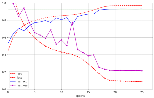
Illustration 2 – Convergence to val_ac = 0.9287 / 0.9303 (at epochs 20 / 22, respectively) for run 34 with WD=0.15
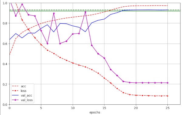
Illustration 3 – Convergence to val_ac = 0.9286 (at epoch 20) for run 45 with WD=0.17
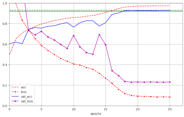
Illustration 4 – Convergence to val_ac = 0.9263 / 0.9302 (at epochs 20/25) for run 3 with WD=0.19
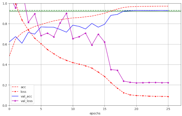
Illustration 5 – Convergence to val_ac = 0.9270 / 0.9316 (at epochs 20/25) for run 61 with WD=0.25
Very satisfying!
Sometimes convergence at epochs > 20 for mixed precision runs
The table above does not display all runs I have performed. The situation, therefore, is not so clear as it my appear from the table above. Really good results depend a bit on the results of statistical weight initialization (HeloNormal sometimes produces high values) and on the statistically selected images for the validation data set (stratification is not always perfect). And on “mixed precision“.
Roughly 25% to 30% of the mixed-precision runs for the same LR-schedule will give you values just close to 0.92 (slightly below or above) at epoch 20, even for otherwise seemingly optimal parameters. In particular for LR-schedule 2 and WD > 0.20. Not withstanding a possible convergence to the threshold value of val_acc =0.92 ahead of epoch 25. This kind of statistics seems to be significantly better for 32-Bit runs (< 5% for not reaching 0.92 at epoch 20).
In general I have to say: Consistently good results (with very, very few exceptions) were achieved with 32-Bit variable precision. In addition, my impression was that the size of fluctuations in val_loss were in general smaller for 32-Bit runs than for mixed-precision runs. For some mixed-precision runs amplitudes of 4 were reached for WD=0.25.
All in all I got the impression that for very short runs to achieve “super-convergence” we should use 32-Bit runs. Meaning, that for super-convergence we should also accept a somewhat higher energy consumption (< 100 Watt on a 4060TI throughout the training runs) .
Fluctuations of the validation loss?
In my previous posts I emphasized the occurrence of fluctuations with relatively high amplitudes in the validation loss. I got such fluctuations again – especially for high values of WD > 0.19. The next 2 images give examples:
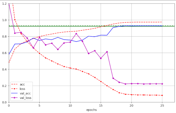
Illustration 6: Large scale fluctuation of the validation loss for a large WD=0.20 (run 56)
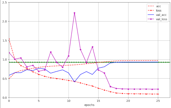
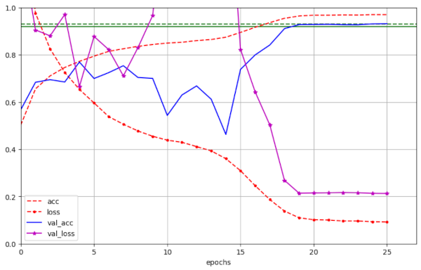
Illustration 7: Large scale fluctuation of the validation loss for a large WD=0.25 (run 57)
However, for WD ≤ 0.19 fluctuations in general become smaller, with a few exceptions.
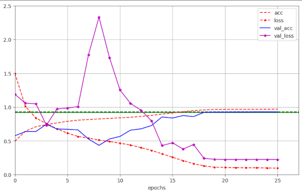
Still, we see maximum values of val_lossmax = 1.2 also there. I should mention that for mixed-precision runs and WD=0.25 a few times amplitudes of val_loss > 4 were reached. This did not affect the final validation accuracy, though.
Illustration 8: Fluctuation of the validation loss for a large WD ≤ 0.19 (run 4)
Compare these examples to plots in previous runs!
Results for combined changes 1, 2 and 3
Below you find the results for all changes combined. All runs done with 32-Bit accuracy. I found consistently that if we use activation for the shortcut Conv2D layer, then we should also use Batch Normalization [BN]. I have, however, not listed all respective test runs in the table below. You just have to accept the message …
I got the impression that the fluctuations were in general somewhat smaller than for the runs in table 1. Regarding validation accuracy I did not see much improvement. But, I admit that I have not investigated this in more detail. Neither did I try out “mixed precision” runs.
Table 2 – runs up to 25 epochs – with all changes in place
| # | epoch | acc_val | acc | epo best | val acc best | final loss | final val loss | shift | l2 | λ | α | LR reduction phases | Remark |
| 8 | 21/22 | 0.91990 0.92020 | 0.9714 0.9733 | 24 | 0.92260 | 0.0804 | 0.2438 | 0.07 | 0.0 | 0.19 | 8.e-4 | [8.e-4, 0]lin[1.0e-3, 5]lin[1.0e-3, 10]cos[1.e-5, 20]lin[8.e-6, 26] | Changes 1, 2, 3 No BN for shortcut |
| 9 | 20 | 0.92080 | 0.9645 | 25 | 0.92260 | 0.0899 | 0.2373 | 0.07 | 0.0 | 0.19 | 8.e-4 | [8.e-4, 0]lin[1.0e-3, 5]lin[1.0e-3, 12]cos[1.e-5, 20]lin[8.e-6, 26] | Changes 1, 2, 3 No BN for shortcut |
| 10 | 19 | 0.92300 | 0.9615 | 24 | 0.92650 | 0.0761 | 0.2255 | 0.07 | 0.0 | 0.19 | 8.e-4 | [8.e-4, 0]lin[1.0e-3, 5]lin[1.0e-3, 12]cos[1.e-5, 20]lin[8.e-6, 26] | Changes 1, 2, 3 BN for shortcut enabled ! |
| 11 | 19 | 0.92490 | 0.9640 | 23/25 | 0.92820 0.92860 | 0.0806 | 0.2221 | 0.07 | 0.0 | 0.19 | 8.e-4 | [8.e-4, 0]lin[1.5e-3, 4]lin[1.5e-3, 8]cos[1.e-5, 20]lin[7.e-6, 26] | Changes 1, 2, 3 BN for shortcut enabled ! |
| 12 | 19 20 | 0.92350 0.92620 | 0.9577 0.9616 | 22 | 0.92650 | 0.1008 | 0.2238 | 0.07 | 0.0 | 0.19 | 8.e-4 | [8.e-4, 0]lin[2.0e-3, 4]lin[2.0e-3, 8]cos[1.e-5, 20]lin[7.e-6, 26] | Changes 1, 2, 3 BN for shortcut enabled ! |
| 13 | 19 | 0.92290 | 0.9556 | 23 | 0.92410 | 0.1029 | 0.2305 | 0.07 | 0.0 | 0.19 | 8.e-4 | [8.e-4, 0]lin[2.0e-3, 3]lin[2.0e-3, 7]cos[1.e-5, 20]lin[7.e-6, 26] | Changes 1, 2, 3 BN for shortcut enabled ! |
| 14 | 19 20 | 0.92440 0.92650 | 0.9626 0.9676 | 22 | 0.92760 | 0.0876 | 0.2215 | 0.07 | 0.0 | 0.20 | 8.e-4 | [8.e-4, 0]lin[1.5e-3, 4]lin[1.5e-3, 8]cos[1.e-5, 20]lin[7.e-6, 26] | Changes 1, 2, 3 BN for shortcut enabled ! |
| 65 | 19 20 | 0.92530 0.92780 | 0.9629 0.9671 | 22 | 0.92760 | 0.0819 | 0.2206 | 0.07 | 0.0 | 0.22 | 8.e-4 | [8.e-4, 0]lin[1.5e-3, 4]lin[1.5e-3, 8]cos[1.e-5, 20]lin[7.e-6, 26] | Changes 1, 2, 3 BN for shortcut enabled! 32-Bit |
| 15 | 20 | 0.92280 | 0.9620 | 25 | 0.92420 | 0.0997 | 0.2292 | 0.07 | 0.0 | 0.25 | 8.e-4 | [8.e-4, 0]lin[1.5e-3, 4]lin[1.5e-3, 8]cos[1.e-5, 20]lin[7.e-6, 26] | Changes 1, 2, 3 BN for shortcut enabled ! |
| 66 | 19 20 | 0.92490 0.92780 | 0.9603 0.9674 | 25 | 0.92910 | 0.0950 | 0.2140 | 0.07 | 0.0 | 0.25 | 8.e-4 | [8.e-4, 0]lin[1.5e-3, 4]lin[1.5e-3, 8]cos[1.e-5, 20]lin[7.e-6, 26] | Changes 1, 2, 3 BN for shortcut enabled! 32-Bit |
| 67 | 19 20 | 0.92380 0.92860 | 0.9565 0.9652 | 25 | 0.93090 | 0.0890 | 0.2145 | 0.07 | 0.0 | 0.25 | 8.e-4 | [8.e-4, 0]lin[1.0e-3, 5]lin[1.0e-3, 12]cos[1.e-5, 20]lin[7.e-6, 26] | Changes 1, 2, 3 BN for shortcut enabled! 32-Bit |
| 68 | 19 20 | 0.92560 0.92750 | 0.9644 0.9716 | 24 | 0.92840 | 0.0732 | 0.2293 | 0.07 | 0.0 | 0.17 | 8.e-4 | [8.e-4, 0]lin[1.0e-3, 5]lin[1.0e-3, 12]cos[1.e-5, 20]lin[7.e-6, 26] | Changes 1, 2, 3 BN for shortcut enabled! 32-Bit |
| 16 | 18 19 | 0.92300 0.92930 | 0.9589 0.9696 | 22 | 0.93070 | 0.0706 | 0.2163 | 0.07 | 0.0 | 0.15 | 8.e-4 | [8.e-4, 0]lin[1.5e-3, 4]lin[1.5e-3, 8]cos[1.e-5, 20]lin[7.e-6, 26] | Changes 1, 2, 3 BN for shortcut enabled ! |
Illustration 7 – Convergence to val_ac = 0.931 for run 67 with WD=0.25
Conclusion – Super-Convergence for a ResNetV2 with AdamW and pure decoupled weight decay
We got a significant improvement of our ResNetV2 without changing the number of layers. We simply changed the kernel-size of the shortcut Conv2D-layer to (3×3) instead of (1×1) and removed pooling from the fully connected part. By these measures alone we pressed the number of epochs required for convergence down to epoch 20 – for our threshold val_acc=0.92. Almost all performed 32-Bit runs reached this threshold value at epochs 19 or 20.
In addition we got values above 0.924 < val_acc < 0.0931 for around 84% of our 32-Bit runs ahead of epoch 25. We have achieved this result for a still relatively low number of parameter around 2.1 million.
We had obtained similar results only for much longer runs (Nepoch > 50) before (at that time without changes 1 and 2).
Using pre-activation and batch-normalization for the Conv2D-shortcut layers at the very first RU of each Residual Stack is not required. However, if you like to try it out, use Batch Normalization, too.
As we consistently can reproduce our results for certain simple, but balanced LR-schedules and for a range 0.15 < WD < 0.25 I would call this a kind of “super-convergence” for our ResNet56v2 with AdamW. (At least for the CIFAR10 dataset.)
Note, however, that not all results fit with publications on super-convergence achieved with the SGD-optimizer. I also got the impression that one should use 32-Bit- and not “mixed precision” – for short runs. But this should be investigated in more detail.
In the next post we shall try another code improvement: We shall improve the so called “bottle-neck” of the Residual Units.
Links and literature
[1] Rowel Atienza, 2020, “Advanced Deep Learning with Tensorflow 2 and Keras”, 2nd edition, Packt Publishing Ltd., Birmingham, UK
[2] Python code of R. Atienza for the ResNets discussed in [1] at GitHub:
https://github.com/PacktPublishing/Advanced-Deep-Learning-with-Keras/tree/master/chapter2-deep-networks
[3] R. Mönchmeyer, 2023, “ResNet basics – II – ResNet V2 architecture”., blog post on ResNetV2 – Layer structure,
https://machine-learning.anracom.com/2023/11/13/resnet-basics-ii-resnet-v2-architecture/
[4] K.He, X. ZZhang, S. Ren, J. Sun, 2015, “Deep Residual Learning for Image Recognition”, arXiv:1512.03385v1 [cs.CV] 10 Dec 2015, https://arxiv.org/pdf/1512.03385
[5] K.He, X. ZZhang, S. Ren, J. Sun, 2016, “Identity Mappings in Deep Residual Networks”, arXiv:1603.05027v3 [cs.CV] 25 Jul 2016,
https://arxiv.org/pdf/1603.05027