The analysis of face images by a trained Autoencoder and the generation of face images from statistical vectors is a classical task in Machine Learning. In this post series I want to clarify the properties of vector distributions for face images generated by a trained standard Convolutional Autoencoder [CAE] in its latent space. The dataset primarily used is the CelebA dataset.
My claim is that if we leave the mapping of the training images to latent vectors completely to the CAE itself and impose no restrictions on the resulting distribution, we already get a “Multivariate Normal Distribution” [MND] – at least in the case of the CelebA image set [1]. I.e. we talk about a resulting MND in the latent space without having enforced it – in stark contrast to Variational Autoencoders [VAEs] or Gaussian Autoencoders [GAEs].
An unenforced MND has already been seen in previous numerical experiments of Ralph Mönchmeyer with the CelebA dataset [2]. In this series I want to reproduce this result, extend the analysis and test whether and how there are dependencies on the chosen specific image dataset and on some properties of the CAE-network (as e.g. batch normalization).
The posts of this series are part of an ongoing private research on how networks with convolutional layers encode information about face data in a latent space. The author is a retired person with some scientific background in physics. No commercial interests are intended. I would, however, be happy if you quote me and this website when using results I discuss here.
I will not go into the basics of Autoencoders, Variational Autoencoders and convolutional networks. In the next post I will just give a very brief summary of the structure of a standard CAE in connection with the setups I will use for my forthcoming experiments. Mathematical aspects of MNDs – as far as we need them – are discussed in a dedicated parallel post series in this blog.
Previous work on this subject
Two years ago I experimented with the CelebA dataset [1] and a very basic CAE. I primarily wanted to show that you can perform respective generative experiments on a standard Linux PC and even with graphics card of very limited capacity. The question in how far the vector distribution created by a standard CAE differed from the enforced distributions generated by a Variational Autoencoder [VAE] was just a side aspect in the beginning.
Actually, it came as a surprise to me to find that the data distribution generated of a CAE in its latent space for CelebA images appeared to have the form of a confined multidimensional ellipsoid located off-center of the latent space’s coordinate system. I have documented this and further analysis done with the help of a PCA transformation, 2D-projections and spectral decomposition already in a sister blog [2]. My conclusion was that the latent vector distribution, by which my basic CAE encoded face information, formed a MND – at least up to a distance of 3 sigma around the distributions center. The occurrence of a multivariate normal distribution happened without any measures or special layers to enforce a Gaussian encoding. I did not even apply batch normalization layers in the central runs.
Unfortunately, in 2022 I had no capacity left to investigate dependencies on the dataset or specific network settings any further. Neither did I care about the variation of certain defined face features (like gender, black hair or spectacles) within the MND. However, the latter would help to support face morphing or the generation of faces with certain properties via latent space vector arithmetic.
I also have jumped over mathematical aspects of the analysis performed. With this post series and a concurrent series on some math aspects of MNDs I want to close existing gaps and prepare the ground for further analysis.
Results so far
In this section I want to remind you of some already derived results. We regard the created latent vectors as “position vectors” to points in the latent space which we cover with an Euclidean Coordinate System [ECS]. After the training of our CAE, each image is mapped to a point and a respective position vector in the CAE’s latent space.
For my previous experiments I had downsized the CelebA training images to a resolution of 96×96 px, only. The CAE consisted of four convolutional layers both in the Encoder and in the Decoder part. Batch normalization was not used. No special layers as in VAEs or AEs were added. The latent space had 250 dimensions.
Minuscule chances to hit a small, confined region of a high dimensional latent space by statistically generated vectors
Regarding image generation by a trained CAE one typically uses statistically chosen vectors in the latent space as input to the CAE’s Decoder. For a VAE we know that the latent vectors can be chosen to be relatively short and point into a sphere around the ECS origin. Reason: The latent distribution of a VAE is enforced to center and cover a limited range around the origin. But what if a standard CAE creates a confined distribution somewhere off the origin? How are our chances to hit such a region with a statistically created vector?
Answer: The chances are negligible. Reason: The high number of dimensions (> 250) and the resulting vastness of the latent space. Statistics is simply against us in such a situation. I have outlined the mathematical argumentation in two blog posts in [3].
Consequence: If a CAE should produce a confined and relatively dense distribution in its latent space we need information about the location and extension of such a latent distribution. It is natural to assume that any statistical latent vectors used for image generation should at least point into the region of the distribution created for the training images. Otherwise we would probably not be able to create reasonable images by a CAE’s Decoder.
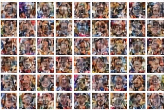
Actually, my CAE produced a confined and dense latent distribution for CelebA off the origin of the latent space’s coordinate system. The failure of creating reasonable face images from freely generated statistical vectors with endpoints within a spherical volume around the origin is shown in the following pictures:
Illustration 1: Failure to create face images based on statistically generated vectors in the latent space of a CAE

Neither a generation of vectors with a constant probability across intervals along the axes nor Gaussian distributions with statistical means and variances along the various axes would help to overcome this difficulty.
Face images from latent vectors pointing into the confined latent space distribution
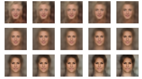
As soon as I uses (statistical) vectors pointing into the confined latent space distribution I got reasonable face images from the Decoder.
Illustration 2: Images created from vectors with endpoints along a line across the ellipsoidal latent space distribution of a CAE

Illustration 3: Images created by statistical vectors pointing into a 3-sigma region of the multidimensional MND ellipsoid

Note that while the successful generation of faces depends on an analysis of the center and the extensions of the latent space distribution the chosen vectors are still statistical in the sense as they do not coincide with points given by the training. The vectors end points ended up statistically within a 3 sigma border surface of the assumed underlying MND.
In the example above the latent space had 250 dimensions, only. And the training images had a relatively low resolution. This accounts in parts for the somewhat unclear images. We also see the weakness in reconstructing reasonable hairdos. However, compare my images to VAE- and GAN-based images published in [4] under similar latent space conditions. The quality improvement is striking.
Maybe, we do not need VAEs or other enforced regularization method at all for face image generation by standard CAEs
In general, it is taught in text books on Machine learning and Autoencoders that the vector distribution in an Euclidean Coordinate System [ECS] of the CAE’s latent spaces may result in both vast, asymmetric, off-center and strange sub-optimal distributions of the vectors’ end-points. This gave rise to an assumed and proclaimed necessity to use VAEs. A VAE enforces an encoding by minimizing the distance to true Gaussians by adding specific layers to the CAE’s Encoder. Another approach was made by adding layers to the CAE which directly enforce approaching a Gaussian cumulative distribution function in the latent space (see e.g. [6]) during training. Such efforts are in particular driven by the efficiency of encoding decisive feature information with very few parameters (mean values and variances).
However, at least for the case of CelebA the above results show that we instead should look beyond text-books and invest some time in the analysis of the unenforced “natural” latent space distribution created by a standard CAE for face images. It might already become a MND without enforcing it. 🙂 . The problems for generative are that the distribution’s center typically would be located somewhere off the origin, that its orientation is rotated in comparison to the axes of the ECS and that the extensions in many of its internal primary axes are not big.
Dense ellipsoidal distributions off the origin of the ECS
In [2] I have shown that projections of the vector distributions generated of a CAE trained on the CelebA dataset on 2D coordinate planes all have ellipsoidal shapes. See the illustration below:
Illustration 4: 3-sigma contours of various projections of the CAE created latent space distributions onto statistically selected coordinate planes

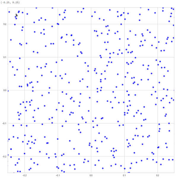
The point distribution appears to be very dense in the illustrations above. However, this is due to the projection of all points distributed over 250 dimensions onto an only 2-dimensional plane. The impression of a high density is also due to a visual scaling effect with respect to the chosen point of view. When you dive deep into the distribution you find void like region – even close to the distribution’s center.
Illustration 5: Close lookup of the 2D-projections near the center

Enough space, still, for statistically chosen points as input for image generation.
If the theory with an underlying MND were correct, we would expect to see elliptic contours of the probability density in all 2-dimensional marginal distributions. The reason is that the marginal distributions of a MND are MNDs of lower dimensionality themselves. In 2-dimensins we get “Bivariate Normal Distributions” with ellipses as contours.
The next plot shows the contours of the point distribution in a chosen coordinate plane vs. theoretical curves for chosen sigma values of an MND which was defined by the numerically derived variance-covariance matrix of the 250-dimensional distribution.
Illustration 6: Numerically derived contours of a 2D-projection vs. different sigma-values for the underlying MND

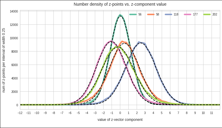
In addition the projections onto the coordinate axes of the latent space can well be approximated by Gaussian functions.
Illustration 7: 1D-projections of the CAE generated latent space distribution onto different chosen coordinate axes and respective Gaussian approximations (dotted lines)

Similar results up to a 3-sigma distance apply to other coordinate planes and coordinate axes. For respective images see the following posts in my other blog on Linux:
- Autoencoders and latent space fragmentation – VIII – approximation of the latent vector distribution by a multivariate normal distribution and ellipses
- Autoencoders and latent space fragmentation – IX – PCA transformation of the z-point distribution for CelebA
Outside the regions for sigma = 2.5, i.e. in the low density tails, the deviations from ideal distributions are sometimes a bit bigger for some coordinate planes and coordinate axes than for the selected cases displayed above. See e.g. the left tail of the orange line in illustration 7. Interestingly, outside a 3-sigma area variations in the background of the original face images dominate the generation of images by the CAE Decoder.
Objectives
When you find a “Multivariate Normal Distribution” in numerical experiments, you, of course, ask yourself what the reasons might be. In particular in my case as I had not used any special measures to ensure a Gaussian-like encoding as it is done in VAEs or GAEs. So, there must be other reasons:
Does it have to do with the properties of the population you pick your samples from? If so, why should a neural network adding filters upon filters in the end detect particular Gaussian patterns in the data? Let us assume that some innermost map of the convolutional neural network [CNN] indeed detects “eyes”. Then it still is a big step to encoding potential Gaussian properties of the eyes distance into a latent dimension for image generation.
Another idea one may get is that the way a CNN works will automatically lead to a MND – if we gave the CNN enough freedom to encode detected properties – i.e. if we offered enough dimensions of the latent space and/or if we provide enough layers or maps. Some theoretical efforts have been made in this direction (see e.g. [6]), but are, in my opinion, far from a convincing proof. While we know that the Central Limit Theorem plays a role in fully connected MLPs, the situation is much more intricate and complex in the case of filtering CNNs.
I will not yet try to answer such interesting questions – in particular because building a solid line of mathematical argument appears to be difficult. One reason is the complexity which the dependencies of the maps in the different successive convolutional layers impose on a mathematical description and analysis of the forward transport between layers (see [6]). Instead, I want to make further numerical experiments to get onto more solid ground regarding the creation of a multivariate normal distribution from face images.
Objective 1 – reproduction of previous results: My experiments in 2022 and 2023 were done with a very simple CAE based on 4 convolutional layers (Keras Conv2D-layers) with a reasonable distribution of the number of maps and a standard kernel-size of (3×3). The chosen activation function was “LeakyReLU”. We should at least vary the number of maps and neurons a bit – and try to reproduce the basic results for CAE based on layers of Keras3. Something which I also will try is to change the initial resolution of the images from 96×96 to 128×128. The impact of the activation function should also be studied.
Objective 2 – impact of batch normalization layers: My previous runs were performed without batch normalization [BN]. Some readers had the suspicion that batch normalization layers in the CAE had induced a tendency of encoding the basic properties of the images in form of a MND. This was not the case. However, it is still interesting to see whether BN has any impact on the result itself.
Objective 3 – impact of the number of latent space dimensions: Another question is whether the number of dimensions of the latent space have an impact on the distribution created by the CAE’s Encoder. There are two aspects:
- a) Does the “Central Limit Theorem” play a role in some peculiar and not really understood way also in CNNs? If this were true we should see something like a MND arising for very different datasets (e.g. MNIST datasets), too, for a growing number of latent space dimensions and/or maps.
- b) On the other side, too many latent space dimensions may hamper the generalization abilities of the CAE – and become counterproductive for image generation. This could show up in a destruction of the ellipsoids for lower sigma values.
Objective 4 – clarify dependency on the CelebA dataset itself: Celebrity faces are peculiar. The selection of persons as “celebrities” may be due to some (unconsciously applied) “beauty attributes” like a pronounced symmetry, relatively narrow Gaussian variations around mean human face features and so on. This may have an impact on the analysis of the neural network. So, what happens if we add non-celebrity faces to the dataset?
Objective 5 – analyze the distribution of certain face features within the MND: A VAE distributes the properties of certain face features (hair color, gender, spectacles, moustache, …) in a way usable for latent space arithmetic. I want to find out how a standard CAE organizes this kind of feature information within the created latent MND.
Objective 6 – a look into the innermost maps of the CAE’s Encoder: In the early phases of image processing by CNNs (between 2009 and 2016) a look at the patterns to which certain maps of the networks reacted sensitively gave some spectacular insights into features and patterns which convolutional networks detected in images during training by applying sequential filters. Therefore, I think it would be interesting to have a look at the specific input pattern to which the innermost maps of the CAE’s Encoder react with large amplitudes of its output averaged over the map’s neurons.
Conclusion
The generative reconstruction of face images by a CAE is interesting as it poses questions about the distribution of vectors in the latent space filled by an Encoder. Previous results for very basic CAEs indicate a MND, at least for CelebA images – without having applied any related measures or specific layers enforcing Gaussian encoding. This may not have been seen and discussed by other authors, because the MNDs are very confined and reside off the origin of the coordinate system with a peculiar orientation of the main MND axes. Therefore, unenforced MNDs resulting from CAEs applied to face images is worth further investigations.
In the next post I will briefly describe details of the setup of the neural networks used in my forthcoming experiments.
Links
[1] CelebA dataset – for the original set see https://mmlab.ie.cuhk.edu.hk/ projects/ CelebA.html.
Another download options are provided at https://www.kaggle.com/ datasets/ jessicali9530/ celeba-dataset and at https://www.tensorflow.org/ datasets/ catalog/ celeb_a
[2] Ralph Mönchmeyer, 2023, post series on the latent space distribution created by a standard CAE for CelebA data
- Autoencoders and latent space fragmentation – X – a method to create suitable latent vectors for the generation of human face images
- Autoencoders and latent space fragmentation – IX – PCA transformation of the z-point distribution for CelebA
- Autoencoders and latent space fragmentation – VIII – approximation of the latent vector distribution by a multivariate normal distribution and ellipses
- Autoencoders and latent space fragmentation – VII – face images from statistical z-points within the latent space region of CelebA
- Autoencoders and latent space fragmentation – VI – image creation from z-points along paths in selected coordinate planes of the latent space
- Autoencoders and latent space fragmentation – V – reconstruction of human face images from simple statistical z-point-distributions?
- Autoencoders and latent space fragmentation – IV – CelebA and statistical vector distributions in the surroundings of the latent space origin
- Autoencoders and latent space fragmentation – III – correlations of latent vector components
- Autoencoders and latent space fragmentation – II – number distributions of latent vector components
- Autoencoders and latent space fragmentation – I – Encoder, Decoder, latent space
[3] Ralph Mönchmeyer, 2023, posts on statistical vectors in the latent space and the probability to hit confined regions,
- “Latent spaces – pitfalls of distributing points in multi dimensions – I – constant probability density per dimension“,
- “Latent spaces – pitfalls of distributing points in multi dimensions – II – missing specific regions“
[4] D. Foster, 2023, “Generative Deep Learning”, 2nd ed., chapters 3 and 4, O’Reilly, Sebastopol, CA
[5] J. Duda, 2019, “Gaussian Autoencoder”, arXiv:1811.04751v4 [cs.LG] 14 Jan 2019, https://arxiv.org/pdf/1811.04751
[6] A. Borovykh, 2019, “A Gaussian Process perspective on Convolutional Neural Networks”, arXiv:1810.10798v2 [stat.ML] 9 Jan 2019, https://arxiv.org/pdf/1810.10798