Among other thins this post series is about efforts to reduce the number of training epochs for ResNets. We test our ideas with a ResNet applied to CIFAR10. So far we have tried out rather simple methods as modifying the schedule for the learning rate [LR]. In this post I describe experiments regarding a model using the AdamW optimizer, without any L2-regularization, but with varying weight decay. We will see that a sufficiently large weight decay parameter λwd triggers large oscillatory fluctuations of the validation loss ahead of a final convergence phase, but nevertheless gives us a good validation accuracy after a training over only 30 epochs.
Short review of previous experiments
In the first two posts of this series
AdamW for a ResNet56v2 – I – a detailed look at results based on the Adam optimizer
AdamW for a ResNet56v2 – II – linear LR-schedules, Adam, L2-regularization, weight decay and a reduction of training epochs
we have studied a network with 1.7 million parameters trained on the CIFAR10 dataset. We changed the LR schedule from a piecewise constant one to a shortened and piecewise linear schedule. We found that activating a rather small amount of so called “weight decay” in the Adam/AdamW optimizers was helpful to keep up the level of validation accuracy during training over a reduced amount of epochs. With the help of the named measures we brought the number of required epochs Nepo for a validation accuracy of 0.92 ≤ val_acc ≤ of 0.93 down from above 100 to 50:
0.92 ≤ val_acc ≤ 0.93 <=> Nepo < ≈ 50
We got the impression that the Keras implementations of Adam and AdamW handle “weight decay” in the same way.
A rather theoretical excursion in a third post
AdamW for a ResNet56v2 – III – excursion: weight decay vs. L2 regularization in Adam and AdamW
has prepared us for experiments without any L2-regularization, but with (strong) pure weight decay.
Model setup
For the experiments described below I have used the same model setup for a ResNet56v2 as described in post I (layer structure according to R. Atienza, see [1]) with around 1.7 million trainable parameters. This is a relatively low number compared to a model referenced in [8] (branched ResNet with 11.6 million parameters). Probably, also the wide ResNet used in [6] had more parameters.
I deactivated L2-regularization for all model layers. Instead, I activated (pure) weight decay by providing a parameter λwd > 0 to the interface of the AdamW optimizer class (of Keras). The training runs lasted over a maximum of 60 epochs, breaking an accuracy threshold of 0.92 <≈ val_acc <≈ 0.93 at or below epoch 50 and in with a shortened LR schedule even at epoch 30.
I want to underline that I used the Keras implementation of AdamW. Please note that this implementation may deviate from what is done in PyTorch optim and other reference implementations as e.g. of fast.ai. See here. (Personally, I have not yet verified whether the assertions on the different implementation are really true. In addition, I cannot find any distinct statement regarding the application of a decoupled weight decay ahead or before weight update in the text of [8]. To me it just says: Do it decoupled.)
We call the initial learning rate “α”, the weight decay factor “λ” and the ema momentum “m“. “LR” abbreviates “Learning Rate”. The neural network was created with the help of Keras and Tensorflow 2.16 on a Nvidia 4060 TI (CUDA 12.3, cuDNN 8.9). All test runs were done with a batch size BS=64 and image augmentation during training with shifts and horizontal flip. Without augmentation the accuracy values discussed below can not be achieved. Most of the experiments in this post were done with a Keras “mixed precision” policy to reduce energy consumption. Tests performed ahead and intermediately showed no significant deviation from full 32 bit runs.
Open questions to be investigated
As we have seen in the preceding post, L2-regularization and weight decay are equivalent for the SGD optimizer, but not for Adam. In contrast to the standard Adam algorithm, AdamW works with an explicit term controlling weight value reduction in proportion to the present weight at each iteration step for weight update. AdamW, after 2018 has become quite popular (see [4], [6] and [9]). We assume that the direct shrinking the weight values via a weight decay term improves the ability of the network to generalize. But are there other differences?
From numerical experiments we know that the classic L2-regularization adds a certain noise level to the loss, which also raises the final loss value reached at the end of the training. Pure weight decay, instead, primarily accelerates the reduction of weight values – without a direct impact on the shape of the loss function around a minimum and the minimum value itself.
What effects do these differences have on the validation accuracy? What is the impact on the evolution of the validation loss during training? This post will give an answer and show that the evolution of the training loss and the validation loss may differ significantly for a long series of epochs – without hampering the final accuracy values!
We will show that pure weight decay (in the Keras implementation) triggers large fluctuations of the validation loss (accompanied by a temporary reduction of the validation accuracy), as long as the learning rate is relatively big. We will learn that a systematic reduction of the learning rate to very low values is required to harvest positive effects of the fluctuations for validation and test accuracy.
In most key publications which discuss the AdamW optimizer the evolution of the validation loss has not been shown. This post provides respective plots. They contain valuable information about partially extreme fluctuations induced by weight decay during phases of still relatively high, though decaying values of the learning rate.
ResNet56v2 with AdamW and a piecewise linear LR schedule, but without L2-regularization
I performed a first series of test runs to study the effect of varying values of the weight decay parameter λ (= λwd / α ). But sometimes I also changed the initial learning rate α, the LR schedule and the momentum parameter m. Regarding the tables below I use the same notation as in the preceding posts. Note that the λ value used here corresponds to the λwd used in the discussion of the preceding post in this series, but modified by a factor 1/α (see below).
Table 1 summarizes some key results of the first set of runs. Most of these runs were done with an initial learning rate of
- α = 8.e-4.
Table 1: Runs with initial LR=8.e-4
| # | epoch | acc_val | acc | epo best | val acc best | final loss | final val loss | shift | l2 | λ | m | α | reduction model |
| 0 | 47 | 0.91230 | 0.9898 | 60 | 0.91290 | 0.0251 | 0.3374 | 0.07 | 0.0 | 0.00 | 0.98 | 8.e-4 | [8.e-4, 20][8.e-5, 40][1.e-5, 50][4.e-6, 60] |
| 1 | 49 | 0.91810 | 0.9917 | 54 | 0.91910 | 0.0219 | 0.3358 | 0.07 | 0.0 | 5.e-4 | 0.98 | 8.e-4 | [8.e-4, 20][8.e-5, 40][1.e-5, 50][4.e-6, 60] |
| 2 | 51 | 0.91490 | 0.9927 | 56 | 0.91580 | 0.0212 | 0.3312 | 0.07 | 0.0 | 4.e-3 | 0.98 | 8.e-4 | [8.e-4, 20][8.e-5, 40][1.e-5, 50][4.e-6, 60] |
| 3A | 49 | 0.91720 | 0.9923 | – | 0.91720 | 0.0203 | 0.3335 | 0.07 | 0.0 | 0.01 | 0.98 | 8.e-4 | [8.e-4, 20][8.e-5, 40][1.e-5, 50][2.e-6, 60] |
| 3B | 42 | 0.92230 | 0.9915 | 58 | 0.92620 | 0.0139 | 0.2822 | 0.07 | 0.0 | 0.05 | 0.98 | 8.e-4 | [8.e-4, 20][8.e-5, 40][1.e-5, 50][4.e-6, 60] |
| 4 | 44 | 0.92460 | 0.9910 | 51 | 0.92620 | 0.0129 | 0.2709 | 0.07 | 0.0 | 0.09 | 0.98 | 8.e-4 | [8.e-4, 20][4.e-4, 30][8.e-5, 40][1.e-5, 50][2.e-6, 60] |
| 5 | 40 51 | 0.92010 0.93160 | 0.9864 0.9954 | 55 | 0.93320 | 0.0130 | 0.2525 | 0.07 | 0.0 | 0.10 | 0.98 | 8.e-4 | [8.e-4, 20][4.e-4, 30][1.e-4, 40][1.e-5, 50][2.e-6, 60] |
| 6 | 41 | 0.92160 | 0.9878 | 52 | 0.92840 | 0.0121 | 0.2645 | 0.07 | 0.0 | 0.10 | 0.99 | 8.e-4 | [8.e-4, 20][8.e-5, 40][1.e-5, 50][5.e-6, 60] |
| 7 | 42 50 | 0.92080 0.93070 | 0.9896 0.9958 | 54 | 0.93320 | 0.0126 | 0.2520 | 0.07 | 0.0 | 0.11 | 0.98 | 8.e-4 | [8.e-4, 20][4.e-4, 20][8.e-5, 40][1.e-5, 50][2.e-6, 60] |
| 8 | 45 50 | 0.92790 0.93190 | 0.9903 0.9950 | 58 | 0.93300 | 0.0141 | 0.2404 | 0.07 | 0.0 | 0.15 | 0.98 | 8.e-4 | [8.e-4, 20][8.e-5, 40][1.e-5, 50][4.e-6, 60] |
| 21 | 46 50 | 0.92490 0.93380 | 0.9896 0.9937 | 59 | 0.93650 | 0.0162 | 0.2211 | 0.07 | 0.0 | 0.20 | 0.98 | 8.e-4 | [8.e-4, 20][8.e-5, 40][1.e-5, 50][2.e-6, 60] |
| 9 | 49 53 | 0.92850 0.93180 | 0.9878 0.9938 | 59 | 0.93490 | 0.0202 | 0.2279 | 0.07 | 0.0 | 0.25 | 0.98 | 8.e-4 | [8.e-4, 20][8.e-5, 40][1.e-5, 50][4.e-6, 60] |
| 10 | 49 52 | 0.92150 0.93210 | 0.9899 0.9922 | 52 | 0.93210 | 0.0249 | 0.2226 | 0.07 | 0.0 | 0.30 | 0.98 | 8.e-4 | [8.e-4, 20][8.e-5, 40][1.e-5, 50][2.e-6, 60] |
| 11 | 50 | 0.92080 | 0.9825 | 60 | 0.92610 | 0.0481 | 0.2290 | 0.07 | 0.0 | 0.40 | 0.98 | 8.e-4 | [8.e-4, 20][8.e-5, 40][1.e-5, 50][2.e-6, 60] |
For the final values of the loss (training data) and the validation loss (validation data) I have picked the lowest values reached before the respective loss went up again. In all of the following plots the solid green line marks the threshold of val_acc=0.92 and the dotted green line of val_acc=0.93.
Obviously, we need a sufficiently high λ value (λ ≥ 0.05) to cross our threshold line ahead of epoch 50. But we can even reach maximum values of val_acc =0.93 after epoch 50 as run nr. 5 in the table proves.
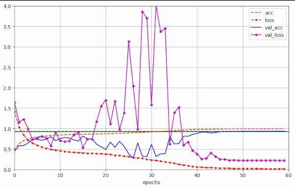
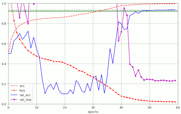
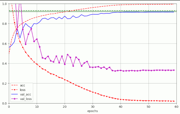
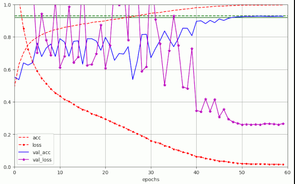
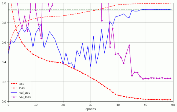
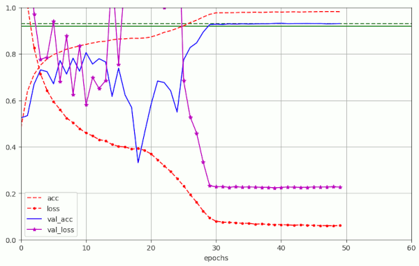
Plot for run nr. 5 with λ = 0.10 – reaching val_acc 0.932 at epoch 51:
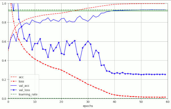
Note the occurrence of oscillatory fluctuations in the evolution of the validation loss during a first phase of constant learning rate up to epoch 20 and during a phase of LR reduction to LR = 1.e-4, reached at epoch 40. In comparison to what we will see below for bigger λ-values, the amplitudes of the fluctuations remain limited to a range of
Note in addition the extremely low value of the eventual loss. This is different from what we experienced in experiments with L2 regularization. See for comparison the plots in the first two posts of this series. I will discuss this point in more detail in a separate section below.
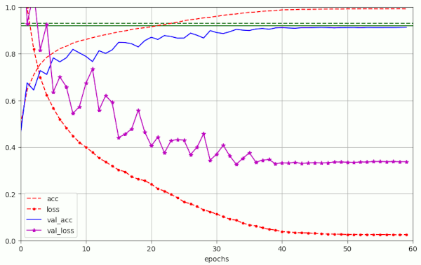
Run Nr. 6 shows that also the momentum parameter m can play a role in failing to reach optimal accuracy values (≥ 0.93).
Plots for run nr. 6 with λ = 0.10 – reaching val_acc=0.9216 at epoch 41, but staying below 0.9284 :

A similar LR schedule as for run 6 has also be used in runs 1-3, 8-11 – with some variation in the final LR-value reached at epoch 60.
Optimal runs reach val_acc = 0.93 before or close to epoch 50
The runs nr. 7, 21, 9 and 10 showed that raising the λ-value increased the oscillatory “noise” in the validation loss significantly. But also during these runs accuracy values acc_val ≈ 0.93 were achieved close to epoch 50. In the experiments 7 and 21 at epoch 50, exactly.
| # | epoch | acc_val | acc | epo best | val acc best | final loss | final val loss | shift | l2 | λ | m | α | reduction model |
| 7 | 42 50 | 0.92080 0.93070 | 0.9896 0.9958 | 54 | 0.93320 | 0.0126 | 0.2520 | 0.07 | 0.0 | 0.11 | 0.98 | [8.e-4, 20][4.e-4, 20][8.e-5, 40][1.e-5, 50][2.e-6, 60] | |
| 21 | 46 50 | 0.92490 0.93380 | 0.9896 0.9937 | 59 | 0.93650 | 0.0162 | 0.2211 | 0.07 | 0.0 | 0.20 | 0.98 | 8.e-4 | [8.e-4, 20][8.e-5, 40][1.e-5, 50][2.e-6, 60] |
It is interesting that in these runs the fluctuations in the validation loss got bigger and pronounced during all the epochs up to epoch 30.
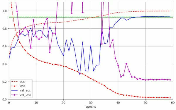
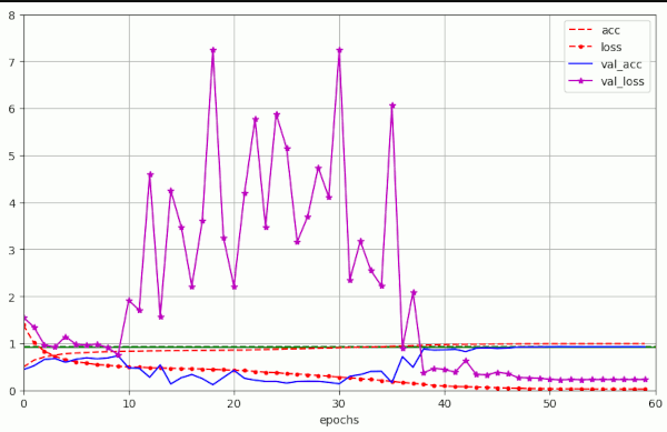
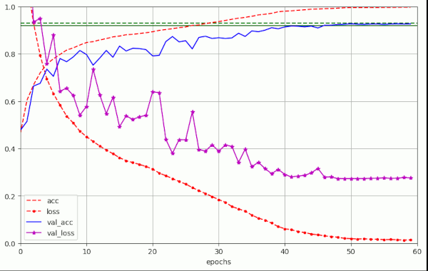
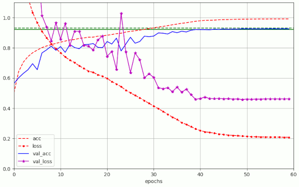
Plot for run nr. 7 with λ = 0.10 – reaching val_acc 0.931 at epoch 50:
(I just have a plot without violet color for the val_loss)
Large scale oscillations
The loss variations in run 7 remained below
However, you find plots with much bigger fluctuation amplitudes
for runs 8 – 10, 21 in further sections below. But this extreme kind of “noise” obviously does not hinder the network to reach good accuracy values within 50 epochs. An example for this somewhat surprising finding is run nr. 21 (see table 2):
The range of optimal λ values for accuracy is limited
The runs 1 to 3A show that we need a minimum of λ ≥ 0.05 to achieve our primary goal. But the numbers in table 1 also indicate that we cannot make λ too big either. Optimal accuracy values – coming with extreme fluctuations (see below) – are reached for 0.1 ≤ λ (= λwd / α ) ≤ 0.3
Thus, for a given LR schedule and a given initial α, the range of optimal weight decay values λ appears to be limited.
Intermediate summary
Using the AdamW optimizer without any L2 regularization in combination with a piecewise linear LR schedule proved to be very effective. From our experiments we conclude that we can achieve our objective of reaching an accuracy level of val_acc=0.92 within 50 epochs. For relatively high values of the λ-parameter (within a limited range) we can even reach val_acc=0.93 close to epoch 50. Which is an improvement of 12.5% of the error rate on the validation data in comparison to experiments of R. Atienza in [1].
Are the values λ for the weight decay not rather big in comparison to L2-parameters?
I have some remarks to make. The first concerns the chosen values of the weight decay parameter λ. The readers who compare the λ-values used above with some values published by the authors of [8] may find a “discrepancy” by roughly a factor of 100 to 400, depending on which parameter set in [8] he/she prefers. The “weight decay values” in [8] cover a range of roughly 1.25e-4 ≤ λ ≤ 5.e-4. The “discrepancy” to λL2 values applied in experiments with L2-regularization in the preceding post for both Adam and AdamW is partially of the same size or even bigger. We need an explanation for this seeming discrepancy.
You may think of the formula for a normalized weight decay given in [8]:
with \(b\) meaning the batch size BS, B the number of training points per epoch and \(T\) the number of training epochs.
But this only gives us a factor of 1 as we have half the batch size and half of the epochs compared to [8]. If you leave out the number of epochs as we do not go to the smallest possible accuracy values we even get a factor around 0.7.
But in my last post we saw that we have to careful regarding the scaling of the λwd-values in comparison to the λL2-values by a factor α. I think this is a very plausible key to the puzzle. When you look at the argumentation of proposition 3 in [8] you come to a regularization effect with a scaled weight decay factor for SGD
(Note that the authors named the weight decay factor w’ instead of the λ we use in this post). If the Keras implementation used a parameter λ in the parameter interface for the constructor of the AdamW class we would come to the right order of magnitude for the weight decay parameter. The rest might be model dependent.
Indeed we find in the Python code for AdamW the parent class TFOptimizer(). There the function to apply weight decay [called weight_decay_fn()] multiplies the user provided weight decay parameter (called “wd” in the code) with the present learning rate (called “lr”). So values 0.09 ≤ λ ≤ 0.2, as we used them in some of the experiments are probably quite reasonable and consistent with the plots shown in [8].
Noise: Large scale fluctuations in the validation loss and validation accuracy
Let us look a bit closer to the evolution of the validation loss and validation accuracy. When we look at the entries in table 1 for the experiments 7 to 10, we see that big values of the weight decay factor λ trigger an improved accuracy. But these relatively big λ-values, together with a relatively the initial LR α, cause really huge fluctuations in the evolution of the validation loss. See the plots below.
The reader may remember that already the plots in the precedent post showed relatively pronounced fluctuations before the learning rate reached a value of η*α = 1.e-4 (with η describing a factor due to the LR schedule). However, as soon as we raise the weight decay factor λ above 0.15 (λ ≥ 0.15) we get really extreme fluctuation amplitudes during the first phase with constant learning rate and the subsequent LR decay phase.
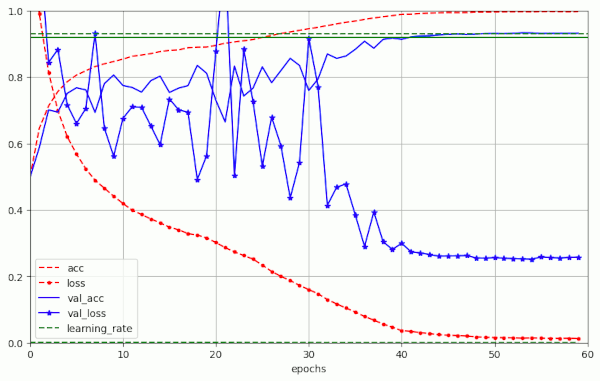
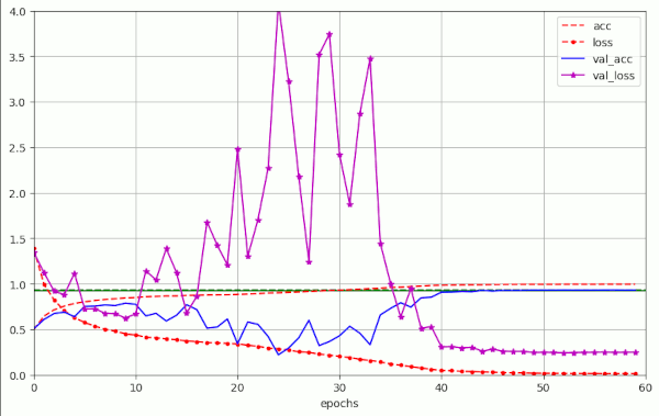
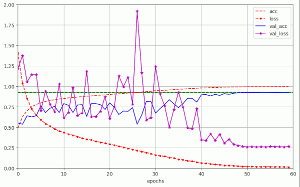
Plot for run 8 with λ = 0.15 – reaching val_acc=0.93 at epoch 50
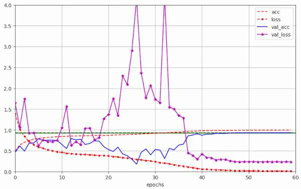
Other extreme examples are the fluctuations for λ = 0.25 and λ = 0.3. Watch the different scales on the y-axis.
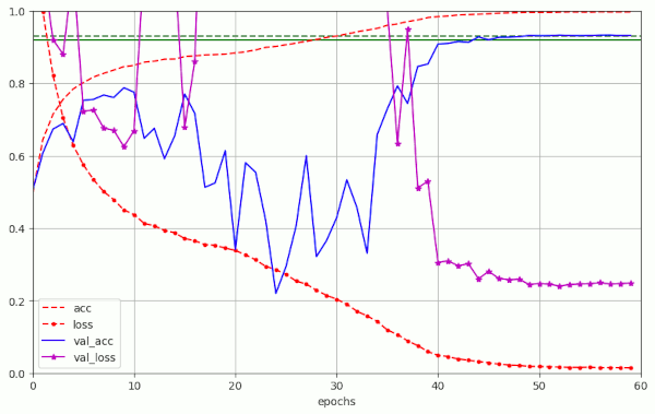
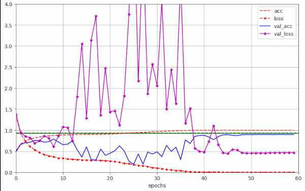
Plot for run 9 with λ = 0.25 – reaching val_acc=0.93 at epoch 52
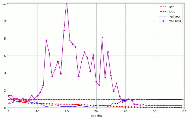
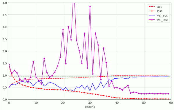
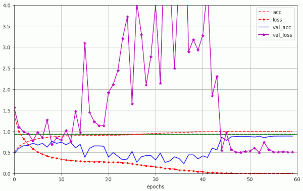
Plot for run 10 with λ = 0.3
Obviously, we drove the amplitudes of the fluctuations into extreme regions. For a physicist this looks like a kind of resonance. The validation accuracy consequently went down to pretty low values for many epochs.
Remarkable discrepancy of the evolution of the training and the validation loss
The fluctuations mark an extreme discrepancy between the evolution of the loss for the training samples in contrast to the evolution validation loss during training. We do not see any such extreme variations for the loss of the training samples during weight optimization.
The discrepancy is extreme between epochs 12 and 35. But as soon as the learning rate drops to 8.e-5 at 40 we get a more continuous evolution. The validation loss than drops rapidly and afterward approaches a constant eventual value relatively smoothly.
Any interpretation must be based on differences between the loss hyper-surface for the validation and the training data over the multidimensional space of the weights. I have given such an interpretation already in the preceding post. I argued that weight decay causes a a constant sideway “drift” in comparison to the model’s gradient descent path. The vector resulting from weight decay corrections points into the direction of the origin of the weight coordinate system and may deviate sometimes strongly from the direction of the loss gradient. In areas of deep and narrow “valleys”
- with small value changes in gradient direction (imagine a river switching direction by 90 degrees),
- but where the gradient changes direction
- and at saddle or bifurcation points
of the loss surface, such sideway movements of the system may lead to collisions with side “walls”. This may happen in the validation loss surface (only) in cases where the “walls” there are located closer to the bottom of the valley than on the loss surface for the training data. It looks at least as if the model is forced by the weight decay drift vector to run up such a steep wall which is closer to the valleys bottom in the val_loss hyper-surface than in the surface of the standard loss. Then it is driven backwards by gradients direction change and up again by the weight decay drift. Such effects may occur until the learning rate drops by orders of magnitude and thus reduces the effects of weight decay in comparison to the remaining loss gradient. I admit that these ideas should be investigated in more detail – both mathematically and by analysis of detailed data about the loss hyper-surface shapes.
Remarkably, the observed resulting decline in validation accuracy to low average values of <val_acc> ≈ 0.2 (!) and 0.4in the experiments 9 and 10 before epoch 40
does not seem to prevent a very good final accuracy result
Special runs to study measures for noise reduction and to check other settings
To investigate some details I performed additional runs with some special settings.
Table 2 – special runs
| # | epoch | acc_val | acc | epo best | val acc best | final loss | final val loss | shift | l2 | λ | m | α | reduction model | comment |
| 12 | 47 | 0.92080 | 0.9912 | 51 | 0.92680 | 0.0127 | 0.2729 | 0.07 | 0.0 | 0.20 | 0.99 | [4.e-4, 20][8.e-5, 40][1.e-5, 50][2.e-6, 60] | smaller initial LR, high WD | |
| 13 | 52 | 0.92080 | 0.9967 | – | 0.92080 | 0.0124 | 0.2955 | 0.07 | 0.0 | 0.13 | 0.98 | 8.e-4 | [8.e-4, 0][4.e-4, 20][2.e-4, 30][8.e-5, 40][1.e-5, 50][1.e-6, 60] | different LR-schedule! |
| 14 | 46 | 0.92030 | 0.9934 | 56 | 0.92560 | 0.0115 | 0.2820 | 0.07 | 0.0 | 0.15 | 0.98 | 8.e-4 | [8.e-4, 0][4.e-4, 20][2.e-4, 30][8.e-5, 40][1.e-5, 50][1.e-6, 60] | different LR schedule! |
| 15 | 50 | 0.92160 | 0.9957 | 55 | 0.92460 | 0.0113 | 0.2839 | 0.07 | 0.0 | 0.20 | 0.98 | 8.e-4 | [8.e-4, 0][4.e-4, 20][2.e-4, 30][8.e-5, 40][1.e-5, 50][1.e-6, 60] | different LR schedule! |
| 16 | 49 | 0.92100 | 0.9933 | 55 | 0.92765 | 0.0134 | 0.2595 | 0.07 | 0.0 | 0.25 | 0.98 | 8.e-4 | [8.e-4, 0][4.e-4, 20][2.e-4, 30][8.e-5, 40][1.e-5, 50][4.e-6, 60] | different LR schedule! |
| 17 | 50 | 0.93110 | 0.9944 | 58 | 0.93430 | 0.0160 | 0.2330 | 0.07 | 0.0 | 0.20 | 0.98 | [8.e-4, 20][8.e-5, 40][1.e-5, 50][2.e-6, 60] | No substraction of mean from samples! | |
| 18 | 50 | 0.93400 | 0.9944 | 56 | 0.93420 | 0.0163 | 0.2281 | 0.07 | 0.0 | 0.20 | 0.98 | 8.e-4 | [8.e-4, 20][8.e-5, 40][1.e-5, 50][2.e-6, 60] | Own stratified validation data, no subtr. of mean |
| 19 | 50 | 0.87943 | 1.0000 | 53 | 0.88686 | 2.5160e-04 | 0.4576 | 0.07 | 0.0 | 0.20 | 0.98 | 8.e-4 | [8.e-4, 20][8.e-5, 40][1.e-5, 50][2.e-6, 60] | No augmentation, own validation set |
| 20 | 50 | 0.87943 | 1.0000 | 57 | 0.89760 | 2.9607e-04 | 0.4944 | 0.07 | 0.0 | 0.20 | 0.98 | 8.e-4 | [8.e-4, 20][8.e-5, 40][1.e-5, 50][2.e-6, 60] | No augmentation, own validation set |
| 21 | 46 50 | 0.92490 0.93380 | 0.9896 0.9937 | 59 | 0.93650 | 0.0162 | 0.2211 | 0.07 | 0.0 | 0.20 | 0.98 | 8.e-4 | [8.e-4, 20][8.e-5, 40][1.e-5, 50][2.e-6, 60] | Optimal run |
Noise reduction by smaller Weight Decay factors of AdamW and by reduced Learning Rate
That the large fluctuations are primarily due to the big λ-values becomes clear when we compare the results of the experiments 9 and 10 with those of run 1 and run 2 in the above table.
Plot for run nr. 2 of table 1 – small weight decay factor λ = 4.e-3, but low accuracy val_acc < 0.915 at epoch 50
A measure which should theoretically help us to reduce fluctuations is a reduction of the initial learning rate α. The following plot shows a run for which the initial LR was chosen to be LR=4.e-4, i.e. half of what we used in the runs discussed in the first sections [8.e-4]. The weight decay parameter was set to a relatively high value again.
Plot for run nr. 12 (see table 2) – big λ = 0.2, smaller α=4.e-4, accuracy val_acc = 0.925 at epoch 50
Regarding accuracy, it seems that a relatively large λ-factor is indeed helpful, even if we damp fluctuations by a reduction of the initial LR α.
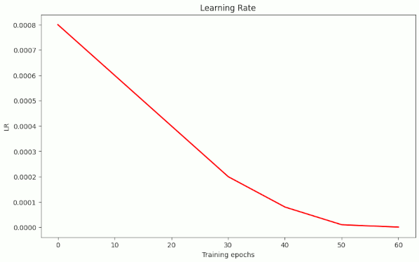
Noise reduction by LR schedule
Very interesting experiments are the runs nr. 13 to 15 because they show that an early phase with a systematic reduction of the learning rate helps to damp fluctuations despite relatively large λ-values.
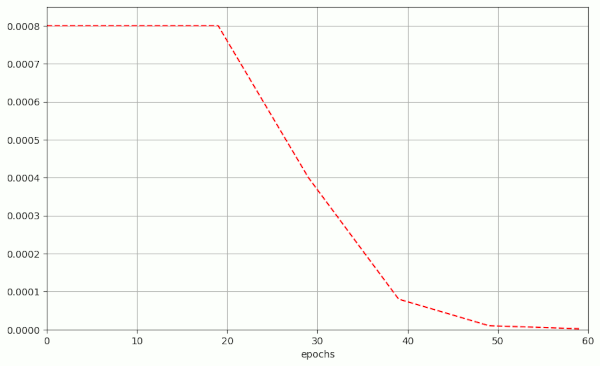
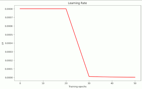
For comparison: Type of learning rate used for the runs in table 1
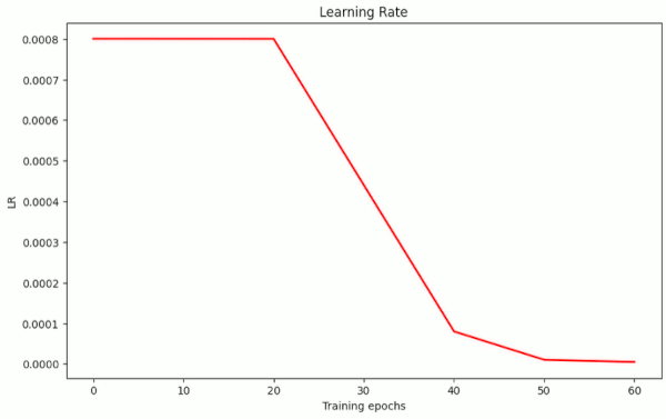
Present decay of the learning rate LR in runs 13 to 15 of table 2 – the values up to epoch 40 are always smaller than for the other LR schedule above
Plot for run nr. 14 (see table 2) – relatively big λ = 0.15, but early LR reduction
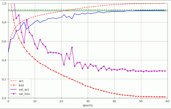
For a critical value of λ = 0.25 we see substantially more oscillatory fluctuations again:
But the maximum amplitude remains below 2.0 – which is significantly smaller than the value 12 which we got for a constant initial LR above in run 10.
So, an early decay of the learning rate indeed does damp fluctuations!
You can read these results in different ways:
- The fluctuations in the first 2 phases of the training depend on a relatively high initial learning rate which has to remain on its high level before it shrinks. A fast reduction of the learning rate by almost two orders of magnitude eventually reduces the noise even for large weight decay values λ.
- A large weight decay value λ is helpful to reach a reasonable accuracy – even if we reduce the learning rate systematically.
- Big weight decay values (λ ≥ 0.2) induce extreme oscillatory fluctuations, i.e. noise, in the validation loss – even if we reduce the learning rate early. It is unclear whether and to what degree this effect depends on specific properties of the CIFAR10 dataset.
- We do not reach optimal validation values val_acc ≥ 0.93 if and when we reduce the learning rate too early.
Point 1 tells us that the observed fluctuations are the result of a combination of a high constant initial LR with a high value of the weight decay factor. Point 4 is an indication that the “noise” induced by high weight decay values in early training phases is helpful to achieve optimal validation and test accuracy values in an eventual phase of convergence to a loss minimum.
Cross checks regarding train and test data
If somebody had presented me the fluctuations of the validation loss without further information, I would have reacted by asking whether something was wrong with the validation data. So, I did some checks on this topic, too.
Run 17 eliminates the subtraction of the mean of the pixel values (of the training data) from both the training and evaluation data to exclude some asymmetry here. The next plot shows that we get the same kind of fluctuations and validation accuracy as we did for other runs with λ ≥ 0.15.
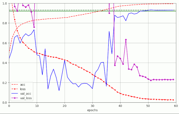
Plot for run 17 with λ = 0.20 – reaching val_acc=0.9311 already at epoch 49 – no centered normalization of the training and test data, but with augmentation
Run nr. 18 repeated run nr. 17, but this time for stratified validation data generated by myself with the help of Sklearn’s function train_test_split(). We get the same size of fluctuations and the same eventual validation accuracy.
Plot for run 18 with λ = 0.20 – reaching val_acc=0.9340 at epoch 50 – with generated stratified validation data set – no centered normalization of the training and test data, but with augmentation
Run nr. 19 shows results for data without augmentation and a newly generated and stratified validation data set. We end up far from the accuracy values with data augmentation, but we observe the same kind of large scale fluctuations.
Plot for run 19 with λ = 0.20 – reaching val_acc=0.89600 at epoch 50 – own stratified validation data set – centered normalization of the data, no augmentation
Run nr. 20 used a different method for the selection and separation of validation data during training. The data were separated by the model.fit() method of Keras itself. This can only be done without using ImageDataGenerator. I used a fraction of 14% of 50,000 samples for validation. But no major changes in comparison to run Nr. 19 could be found. The fluctuations even got a bit worse, because due to selection before shuffling the validation data may not have been sufficiently stratified.
Plot for run 20 with λ = 0.20 – reaching val_acc=0.87943 at epoch 50 – 14% validation samples separated by Keras – centered normalization of the data, no augmentation
Taking all results together they mean means that the observed large scale fluctuations do not result from an accidentally wrong setup of the validation data set.
Summary: The large scale fluctuations in the validation loss are a real effect and they are obviously caused by pure weight decay and respective big values of the parameter λ.
Further reduction of the number of required epochs for val_acc=0.92?
One of my original objectives was the reduction of the number of required epochs for a threshold value of val_acc=0.92. Can we shorten the first phase of extreme fluctuations for relatively high α and λ values? This is indeed possible to a certain degree – even without changing our general strategy for the LR schedule.
Table 3 – Reduction of required number of epochs for val_acc=0.92 to 30
| # | epoch | acc_val | acc | epo best | val acc best | final loss | final val loss | shift | l2 | λ | m | α | reduction model | comment |
| 22 | 35 | 0.92120 | 0.9799 | 44 | 0.93020 | 0.040 | 0.238 | 0.07 | 0.0 | 0.20 | 0.98 | [8.e-4, 20][8.e-5, 30][1.e-5, 40][4.e-6, 50] | big LR, big WD, but shortened 2nd and 3rd LR phase | |
| 23 | 30 35 | 0.92610 0.92950 | 0.9679 0.9792 | 41 | 0.93170 | 0.061 | 0.225 | 0.07 | 0.0 | 0.20 | 0.98 | [8.e-4, 20][1.e-5, 30][4.e-6, 40][2.e-6, 50] | big LR, big WD, but short 2nd LR phase | |
| 24 | 28 | 0.92090 | 0.9650 | 32 | 0.92420 | 0.075 | 0.227 | 0.07 | 0.0 | 0.20 | 0.98 | 8.e-4 | [8.e-4, 18][1.e-5, 28][4.e-6, 36][2.e-6, 40] | big LR, big WD, but very short 2nd LR phase |
| 25 | 27 | 0.92020 | 0.9685 | 30 | 0.92160 | 0.084 | 0.241 | 0.07 | 0.0 | 0.22 | 0.98 | 8.e-4 | [8.e-4, 18][1.e-5, 26][2.e-6, 36] | big LR, big WD, but very short 2nd LR phase |
In run nr. 22 I reduced the 1st phase with constant α = 8.e-4. I hoped that I could reach the threshold value at least within 40 epochs. Actually, we reached our goal already at epoch 35. See the plot below.
Plot for run nr. 22 which reaches val_acc=0.92 at epoch 35 and val_acc=0.930 at epoch 44
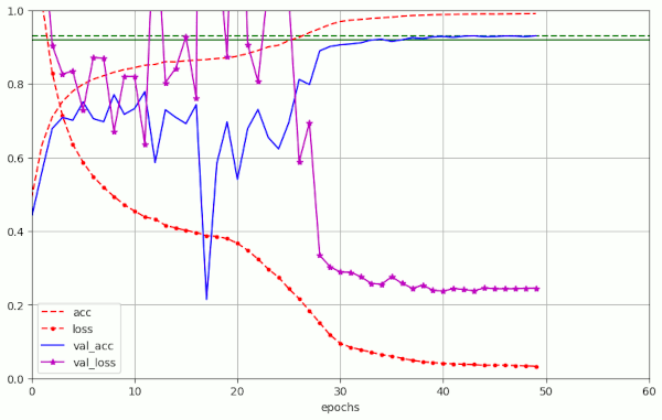
We have a sharp spike at epoch 17, but otherwise we find again that this type of initial noise is no hinder.
The next trial run (nr. 23) was set up to be even shorter. I reduced the learning rate η*α steeply from 8.e-4 to 1.e-5 between epochs 20 and 30. And, surprise: We reached val_acc=0.92610 at epoch 30 and val_acc=0.93090 at epoch 35.
Plots for run nr. 23 which reaches val_acc=0.92 at epoch 30 and val_acc=0.9295 at epoch 35
We can have some doubts whether the run 23 and run 22 converged to the same final solution – as the loss for the training data in run nr. 23 is somewhat higher than the loss in run nr. 22 – and the opposite is true for the validation data. So, we may have a side valley with a local minimum close to a valley that leads to the eralglobal minimum on the loss hyper-surface for the training data.
In experiment nr. 25 I could bring the epoch for our accuracy threshold down to epoch 27. I could not get smaller epoch numbers by my present strategy of an initial phase with a constant and relatively big LR value.
Discussion of the results of our experiments so far
“Noise” in the form of large scale fluctuations of the validation loss during initial phases
What have almost all of the experiments between the posts I, II and the present one in common? Answer: We distinguish a two first phases (with constant large LR) with a lot of noise in the validation loss and the accuracy from an eventual phase with very low values of the learning rate and a fast convergence. For the runs up to 60 epochs we have :
- First phase with constant learning rate LR at a high level (α ≥ 8.e-4). The “noise” starts at some point between epochs 10 and 14 for CIFAR10.
- LR decay phase during which the oscillatory noise in the evolution of the validation loss continues until it eventually gets quickly damped by the LR schedule down to LR values η*α ≤ 1.e-4 – with η indicating the schedule’s factor at that point.
- Convergence phase: A phase where gradient descent quickly approaches a local (global?) minimum at very low values of the learning rate LR (η*α ≤ 6.e-5)
Relatively large weight decay values λ in AdamW in combination with a big initial learning rate α trigger significant fluctuations at some point during the first phase. While the loss on average still drops during the first steps the amplitudes of its fluctuations become really large at around epoch 10 to 15 until η*α drops systematically down to below 8.e-5 > η*α ≥ 1.e-5 at between epochs 40 and 50.
In the phases with the big fluctuation amplitudes we observe a huge gap between the loss of the validation and the loss of the training data. For CIFAR10 this noise can have a positive effect on the eventual accuracy level and diminish the final error rate.
The fluctuations can be damped by an early decay schedule for the the learning rate, but can not be suppressed completely for large values of the weight decay parameter λ. We also got an indication that there is an optimal range of weight decay values λ for a defined initial LR of α = 8.e-4. This should be investigated in more detail in further experiments with a systematic variation of α.
Do the large validation loss fluctuations, induced by weight decay, have a positive effect?
The answer is: Yes. Runs 1 and 2 described in table 1 showed that we have no chance to reach val_acc > 0.92 within epoch 50 with λ-values in the range 5.e-4 < λ < 1.e-2. Remember that we used this range earlier in combination with Adam and AdamW and explicit L2-regularization at the models’ layers. So, for AdamW without explicit L2-contributions we absolutely need larger λ-values, at least:
- λ > 0.05
The most astonishing effect is, however, that the really big fluctuation amplitudes for even larger λ-parameters
- 0.2 <= λ <= 0.3
do not hamper the final accuracy value. The opposite is true:
- In both the experiments 9 and 10 of table 1 we reached values of val_acc> 0.9285 within epoch 50 for λ > 0.15.
- In the experiments 2 to 4 of table 2 we even reached values above val_acc >= 0.93.
The network appears to have come to a better generalization during the wild excursion on the validation data hyper-surface. This is not reflected in the variation of loss and accuracy on the training data which evolve rather smoothly. Note that there is a difference to 1Cycle Learning: By 1Cycle Learning we use a first training phase to trigger a rough ride on the loss hyper-surface for the training data themselves.
Whether we can generalize this result from CIFAR10 to other datasets remains to be seen.
Limited range of weight decay values for optimal accuracy
The experiments in table1 also tell us that α and λ are correlated: For a given initial LR α there is an optimal λ (and maybe also an optimal momentum m). This particular finding is a bit in contradiction to what the authors of [8] claim.
Do we find something similar in literature?
A short review shows that [9] there are experiments for CIFAR10 which show substantial fluctuations in the training loss and the test error for a ResNet34 and an initial phase with constant LR. See section 3 and B4 therein. The plots (Figs. 2,3,10) remind very much of my plots in the 1st post of this series. But note that the authors of [9] stretched their calculation over many more epochs, namely 1000. And the cross-entropy is shown on a logarithmic scale for the training data.
AdamW: Noise by momentum driven overshooting and a big LR, only ?
Just to get a comparison the next plot shows a calculation done with λ = 0 – and no L2-regularization (see run nr. 0 in table 1). AdamW shoud then behave as Adam:
This result confirms that the observed huge fluctuations of the validation loss in the other runs is primarily caused by weight decay and not by the relatively big initial learning rate alone.
L2-regularization raises the minimum value of the validation loss
According to the considerations in the preceding post the eventual loss achieved with Adam and some L2-regularization should have a significantly bigger value than the one we get with AdamW and weight decay. This is indeed the case:
Plot for a run with Adam (!) and a small L2-regularization contribution with λL2 = 8.e-5
You see a similar level of the eventual
- L2-regularization: loss = 0.2 and val_loss = 0.48 => much bigger than with weight decay (see table 1).
also in the plots of the previous posts. Compare this to the eventual values for the training “loss” given in table 1 – they are much, much smaller. See the plots for the runs 1 to 10 in addition.
So, it is a bit strange:
- For AdamW the “pure” weight decay term guarantees that the weights are effectively reduced during training.
- Large weight decay values obviously induce extreme fluctuations in the validation loss (for CIFAR10). This “noise” can only be damped by a fast reduction of the learning rate LR – coming with a reduction of validation accuracy.
- Even a relatively small value for the weight decay λ = 4.e-3 reduces the weight values effectively such that the final loss gets close to a value of the training loss = 0.02.
- Consistently, with theoretical consideration sin the preceding post we have to assume that the momentum part of AdamW only refers to the momentum of the gradients of the unmodified original loss function.
- The impact of an additional L2-regularization contribution in the Adam-based part remains a bit unclear for a growing number of epochs.
Conclusion
In this post we have thoroughly investigated a ResNet56v2 model supported by the AdamW optimizer without explicit L2-regularization for the layer weights. For training a batch size B=64 was used. We have seen that such a model can reach accuracy values of at least val_acc=0.92 and with optimal parameter settings also values val_acc=0.93 within 50 epochs.
We even found that by choosing an earlier decay of the LR to 1.e-5 before epoch 30 allowed us to reach val_acc=0.92 already around and a bit below epoch 30.
These results could be achieved with a piecewise linear schedule. It will be interesting to see whether we get similar fluctuations when we replace our piecewise linear schedule by a continuous following a cosine curve. This will be the topic of the next post:
AdamW for a ResNet56v2 – V – weight decay and cosine shaped schedule of the learning rate
We must be cautious regarding a generalizing of our results: We can not be sure that some of our results are a bit specific for the CIFAR10 dataset. Another open question is whether and to what degree the results also depend on the batch size.
Links and literature
[1] Rowel Atienza, 2020, “Advanced Deep Learning with Tensorflow 2 and Keras”, 2nd edition, Packt Publishing Ltd., Birmingham, UK
[2] A.Rosebrock, 2019, “Cyclical Learning Rates with Keras and Deep Learning“, pyimagesearch.com
[3] L. Smith, 2018, “A disciplined approach to neural network hyper-parameters: Part 1 — learning rate, batch size, momentum, and weight decay“, arXiv
[4] F.M. Graetz, 2018, “Why AdamW matters“, towards.science.com
[5] L. N.. Smith, N. Topin, 2018, “Super-Convergence: Very Fast Training of Neural Networks Using Large Learning Rates“, arXiv
[6] S. Gugger, J. Howard, 2018, fast.ai – “AdamW and Super-convergence is now the fastest way to train neural nets“, fast.ai
[7] L. Smith, Q.V. Le, 2018, “A Bayesian Perspective on Generalization and Stochastic Gradient Descent”
[8] I. Loshchilov, F. Hutter, 2018, “Fixing Weight Decay Regularization in Adam“, arXiv
[9] M. Andrushchenko, F. D’Angelo, A. Varre, N. Flammarion, 2023, “Why Do We Need Weight Decay in Modern Deep Learning?“, arXiv
[10] I. Drori, 2023, “The Science Of Deep Learning”, Cambridge University Press