AdamW for a ResNet56v2 – I – a detailed look at results based on the Adam optimizer

The last days I started to work on ResNets again. The first thing I did was to use a ResNet code which Rowel Atienza has published in his very instructive book “Advanced Deep Learning with Tensorflow2 and Keras” [1]. I used the code on the CIFAR10 dataset. Atienza’s approach for this test example is to use image augmentation in addition to L2-regularization with the good old Adam optimizer and a piecewise constant Learning Rate schedule. For a ResNet56v2 I got a test accuracy of 0.92 to 0.93. (See below for a comparison to Atienza’s numbers).

A problematic aspect of Atienza’s way of controlling the Learning Rate [LR] is that it leads to a rather high number of training epochs (between 90 and 200). This post series is about different ways to reduce these epoch numbers to below 50 and even 30. In particular, I want to test the option of super-convergence via a 1Cycle LR schedule – both with the SGD and the AdamW optimizer.

Objectives of this post series

The objective of this post series is to find some answers to the following questions:

Can one reproduce the published results of Atienza with the plain Adam optimizer?
Can one get down to 50 epochs instead of 100 (or 85; see below) used by Atienza to reach a reasonable validation or test accuracy above 92%?
What would happen if one replaced the Adam optimizer by AdamW (or SGD)?
Can we achieve an even faster convergence with a One Cycle Scheduling [OCS] for the Learning Rate [LR]?

I got interested in respective experiments because the results of others discussed in various publications did not appear to be directly comparable. I wanted my own tests with clear conditions. In the present first post of the series I will answer the first question for a ResNet56v2. The 56 refers to the depth (acc. to Atienza) for which only filtering Conv2D layers have been counted. Note that Keras defines the depth of their ResNet networks a bit differently.

While I use my own code for the ResNet setup, I have parameterized it such that it reproduces the layer structure of Atienza’s models exactly. Thus I could also independently check his published numbers. The 85 epochs mentioned above in brackets have to do with a well reproducible validation accuracy value of 0.92 reached at this point with the Adam optimizer and Atienza’s LR schedule and independent of the used Batch Size [BS] during training.

In this post I will also show plots of the accuracy and loss gained during training for both the CIFAR10 training and validation data. We will see that there is a phase during training where relatively large LR values trigger high spikes in the loss of the validation (or test) data. This makes CIFAR10 really interesting for test scenarios. I will give an interpretation of this effect.

In the second post we will see that objective (2) can indeed be achieved – in alternative ways. Note that 50 epochs is only a half or a third of the number of epochs Atienza had to follow in his runs to achieve similar results for the accuracy. We will in addition see that a properly parameterized AdamW does not need any L2-regularization and reaches an even better accuracy. We will the compare the results of AdamW based runs to experiments with the SGD optimizer. A further post will investigate the conditions for the so called “super-convergence” with a kind of 1Cycle LR scheduling scheme. And we will press down the convergence rate even further.

Tensorflow 2.16 – remarks on warnings and the ImageDataGenerator() for augmentation

I use Tensorflow 2 [TF2] and Keras 3 to build my Deep Learning models. At the time of writing TF 2.16.1 is the present Tensorflow version. However, it comes with warnings for using the ImageDataGenerator() functionality to prepare and preprocess images. In the case of CIFAR10 for augmenting the images.

For the CIFAR10 dataset it is well known that augmentation is a necessary ingredient in Deep Learning experiments if you want to achieve high values of the validation accuracy. Typically, you will get an error rate below 10% without augmentation. Therefore, I have performed most of the test runs in this post series with data augmentation. However, this will lead to warnings with TF2.16.1.

You can avoid periodic warnings during training by not setting the parameter “steps_per_epoch” of the model.fit() function explicitly. Omitting this parameter does not cause any harm, as the required value is calculated internally.

Another reason for warnings is that ImageDataGenerator() is regarded deprecated in Keras 3. But it still works! Note however that using it reduces the overall performance because image handling is done intermittently on the CPU. I nevertheless applied it for the test runs of this post. I will show how to replace ImageDataGenerator() by preprocessing layers of Keras models in another post.

Own code, but same model and layers as used by Atienza

We need a clear base for later comparisons between results for different optimizers and Learning Rate schedulers. A ResNet56v2 is well defined by its Residual Stacks and the structure of its Residual Units. This includes the specification of its Convolutional Layers, Batch Normalization, Activation functions and the number of filters per Conv2D layer. See another post of this blog for details. For the purposes of this post series I strictly follow the ResNet setup recipe of Atienza. See his code at this link at github.com.

As said earlier I have used my own classes for the setup of ResNets. I wrote my own code for three reasons: (a) I wanted flexibility in creating ResNets with varying numbers of layers in the various Residual stacks. (Atienza has a strict 3/3 setup). (b) Modifications in comparison to what Atienza has suggested were required to compensate for warnings, error messages and requirements of Keras 3 and Tensorflow 2.16. (c) I wanted more flexibility regarding the parameterization of Learning Rate schedulers and parameters to choose between different optimizers and activation functions. However, during this post series I use the same layer structure, activation functions and filter numbers as Atienza. This structure is simple:

Atienza’s structure of the Residual Stacks
We have an input layer section, which is followed by 3 residual stacks, each containing 6 Residual Units:

Residual Stack RS1: 6 RUs – each with a bottleneck structure of 3 layers:
L1 [k=(1×1), nF=16], L2 [k(=3×3), nF=16], L3 [k=(1×1), nF=64)
Residual Stack RS2: 6 RUs – each with a bottleneck structure of 3 layers:
L1 [k=(1×1), nF=64], L2 [k(=3×3), nF=64], L3 [k=(1×1), nF=128).
Residual Stack RS3: 6 RUs – each with a bottleneck structure of 3 layers:
L1 [k=(1×1), nF=128], L2 [k(=3×3), nF=128, L3 [k=(1×1), nF=256).

k is the kernel size, nF is the number of filters. The network is rather slim in the sense that it only requires around 1.7 million trainable parameters (1,663,338). This is just twice the number of what was required for the ResNet56v2 definition in [8], which used less filters. Other more state of the art networks use more complicated structures, more filters and thus many more parameters.

This ResNet layer structure is a bit peculiar with respect to raising the number of filters from 16 to 64 during the first residual bottleneck blocks. Other authors use a factor of 2 or 4 for filter reduction in the bottlenecks throughout all stacks.

What should we expect? Atienza’s accuracy numbers …

Below I will call the validation accuracy for the usual 10000 validation data samples of CIFAR10 val_acc. Besides conceptual aspects the main difference to a test accuracy is that val_acc is evaluated already during training. If this worries you, read this article. In our case this intermediate evaluation is useful to better judge the impact of certain hyper parameters, foremost of the Learning Rate values, on accuracy convergence. If you would like to define separate test samples feel free to do so in your own experiments.

For a ResNet56v2 we realistically expect a reproducible test or validation accuracy above or at least close to

val_acc = 92%.

I got this number not only from the Atienza book, but also from [8] and from a publication of Leslie Smith (see [3]) on the impact about different learning parameters and Cyclic Learning Schedules on convergence.

Remarks on the accuracy numbers in Atienza’s book
Atienza used L2-regularization with a fixed default value of l2_param = 1.e-4. The Adam optimizer was combined with a LR-scheduler that reduces the Learning Rate according to a “piecewise constant scheme” over the training epochs. In addition image augmentation was applied to achieve his accuracy results.

The results published in Atienza’s book are based on runs with 200 epochs. Unfortunately he did not give much details on the behavior of the validation loss or acc_val during a training run. The standard Batch Size [BS] he used is BS=32 (according to his code at github).

Basic results of my own test runs for a Batch Size of BS=32

According to my own test runs it is fair to say that the val_acc values between 0.91 and 0.92 are often reached already between the epochs 80 and 100. Values of 0.924 between epoch 90 to epoch 120. Values of 0.925 at around epoch 125, 0.927 at around epoch 165.

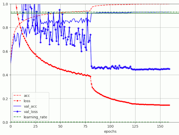
See the plot below where I got no further improvement above the last number. All these numbers were achieved for BS = 32. For other batch sizes see other sections below.

The solid green line marks 0.92, the dotted green line 0.93, which is not reached. Blue lines mark the val_acc and val_loss reached for the validation data. The red lines refer to the development of the accuracy and loss for the training samples.

Results for a run with BS=32 (200 epochs) – reaching val_acc = 0.927

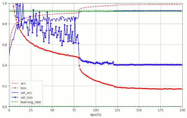
Note the relative abrupt improvement that occurs with epoch 80 at which a reduction of the LR to 1.e-4 takes place. Beyond epoch 125 the improvement of val_acc is only marginal.

A lot of epochs for the last percent in accuracy ..

The above plot basically means:
Around 75 to 100 epochs are used by Atienza’s approach for the last 0.5 to 1.0 percent of improvement in accuracy. These are enormous number that come along with a lot of energy consumption (80W on a Nvidia 4060 TI).

Pronounced spikes in the validation loss for a phase with a relatively big LR

An interesting aspect of the above plot is that

the loss for the training data set evolves relatively smoothly during training
the loss for the validation data set (which is not really small) evolves much more erratically during training.

We will see the same kind of big fluctuations in the validation loss also in other test runs (below in in forthcoming posts). Why is this interesting?

I think it tells us something about the difference between the loss function for the training samples and the validation samples.

Interpretation of the “noise” in the validation loss

Where does all the pronounced noise in the variation of the validation loss “val_loss” come from? In comparison to datasets of other ML problems the depicted variations of the validation loss appear to be a bit extreme … Well, the plot above reminds us about an important fact:

The structure of the loss hyper-surface (vs. the networks weights) for the set of validation samples is similar to the equivalent loss hyper-surface for the samples of the training data samples – but they are not identical!

The reason is that the samples are not the same. In case that the loss surface shows pronounced narrow valleys between very steep walls, already a small shift of the bumpy landscape may have a huge impact. While the gradient on the loss hyperplane may point into the direction along a valley bottom on the hyperplane for the training data, it may lead us up a steep wall on the hyperplane for the validation data. Due to a small shift of the bottom and wall positions for the two datasets.

Regularization also plays a role: For Adam a standard L2-regularization it is less effective in phases when gradients are big and changing fast (see [4] for this point). Shuffling the data produced by the DataImageGenerator() may add to noise in the first phase with .

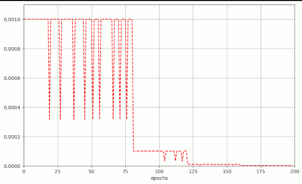
Another point is: The Learning Rate shows remarkable variations. This is due to a callback called ReduceLROnPlateau(). I have skipped this one in my own calculations – or set the minimum rate to a larger value than Atienza.

Formulas?

Some papers have discussed the impact of batch sizes on the fluctuations (“noise level”) of the accuracy and validation accuracy variation during training – in [7] for MNIST data. However, the fluctuations in the evolution of the validation loss for CIFAR10 are seldomly shown – and if so – for much larger batch sizes [3]. L. Smith and Q.E. Le [7] have given a formula to describe a simple scaling rule for the “noise” (= fluctuations) for SGD in [7]. They showed that the noise level in the test/validation accuracy should decrease linearly with the batch size.

\[ g \:\approx\: { \epsilon \, N \over B\, (1\,-\,m)} \]

$g$ is the noise scale, $e$ the learning rate, $N$ the size of training dataset, $B$ the Batch Size and $m$ the momentum.

$g$ The question is whether these dependencies remain true for the Adam optimizer.

Are the named numbers of for the LR scheduler of Atienza reproducible?

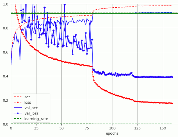
Yes, they are. It could reach the named numbers in three successive test runs. With a variation in the number of epochs of 10 to 15. Below a plot of another run for BS=32, which I stopped at epoch 160 with a val_acc = 0.9265.

Results for a run with BS=32 (over 160 epochs) reaching val_acc = 0.9265

Is a value of val_acc = 0.93 reproducible?

It is not for a batch size of BS = 32. For this batch size a value of v_acc = 0.93 appears to be a selected optimum number which probably is reached during a few runs with Atienza’s scheme. Personally, I never reached it during all in all 5 runs I performed up to epoch 200 over the last days.

An additional remark: Please note that the numbers given for n (n=9) in his table on ResNetv2 models do not fit a Resnet56 but a Resnet83v2.

However:

With a batch size of BS = 64 I once (!) reached it val_acc = 0.9302 at epoch 142. See below for an example graphic. But it varied afterward between 0.929 and 0.9302 for a long time.
For a batch size of BS=128 I multiple times reached val_acc=0.9306 somewhere between epoch 130 and 160. Also then I experienced variations between 0.9293 and 0.9306 for some epochs afterwards.

For respective data see the table given in the section on batch sizes below.

Other observations

Observation 1: LR reduction leads to direct improvements in accuracy

A noteworthy observation is that a reduction of the Learning Rate [LR] in the Atienza schedule always comes with a direct improvement. This leads to the question whether a reasonable scheme for the reduction of the Learning Rate would not give us similar results with a much less number of epochs.

Observation 2: Dependency of accuracy on augmentation and shift parameters

The results on validation accuracy which Atienza published can only be reached with data augmentation. Augmentation is activated in his code via a parameter (which is set to True). The augmentation Atienza used were horizontal and vertical shifts and horizontal flips only. I kept to this policy as it is reasonable for CIFAR10.

Augmentation supports generalization during training. So, this first observation is no wonder. However, it is not so clear what degree of shifting gives you good results. My tests have shown that a shift of 0.07 (7%) to 0.08 (8%) for the maximum shift is an appropriate value. Atienza used 0.1, a value which appeared to be less optimal in my own test runs for a faster LR reduction scheduler.

Observation 3: Impact of the Batch Size on energy consumption

The following numbers a re given for a Ti 4060 and a i7 CPU. Atienza uses the ImageDataGenerator class of Keras for augmentation. This generator got the status “deprecated” with Keras 3. The turnaround times for one epoch were influenced by the generator. One could see this from a pulsing GPU load – which went significantly down between two epochs. The data generator furthermore occupied my 8 CPU-cores (4 + 4 hyperthreads) relatively continuosusly with a certain average load of 30%. Which is significant!

What I have seen so far over various test runs is that the runtime difference for one epoch is not very big if you compare a mini-batch size of BS=128 with a BS=64, namely 20 secs and 22 secs, respectively.

#	BS	best ever acc_val	at epo	GPU	Watt	time per epoch
1	32	0.9273	165	55%	70 W	27 sec
2	64	0.9298	133	71%	97 W	22 sec
3	128	0.9308	164	85%	114 W	20.5 sec

These numbers were observed for standard 32 bit floating point accuracy. The “time per epoch” includes the time for ImageDataGenerator()” and the time for loss and accuracy evaluation on the validation dataset (with 10,000 samples).

When you go down from BS=64 to BS=32 the run-time goes up from 22 secs to 27 secs per epoch (on average and a bit depending on other activities on the system). This is mainly due to a worsening ratio of time spent in the CPU for the generation for augmented images via ImageDataGenerator() vs. time spent in the GPU.

This means that we pay a higher price for saved time. While the power consumption is proportional regarding time saving for BS=32 and BS=64, it is getting worse for BS=128. We only save a little time per epoch, but the power consumption goes up to 114 W.

Reduction of Power Consumption by using “mixed precision”

Keras 2 and Keras 3 allow the usage of a mode in which certain operations (matrix multiplications etc.) can be performed with 16bit accuracy, whilst other important data as the weights are kept in 32bit accuracy. Latest Tensorflow installation in combination with present CUDA and cuDNN versions only do part of this automatically. You still have the option to choose a global Keras policy for the layers by including the following statement in your program before building your Keras DNN models:

tf.keras.mixed_precision.set_global_policy(“mixed_float16”)

See the Keras 3 documentation for more details. This step will bring power consumption down to 65W, only, for BS=64. The acceleration effect, however, is small. We go down from 22 secs to 19 secs per epoch. Part of it is due to the augmentation. Without augmentation by the ImageDataGenerator() we go down to 14secs.

I have taken care by comparison runs that the use of mixed precision only has a negligible impact on the results presented in this post series..

Observation 4: Impact of the Batch Size on run time

Numbers for “transition epochs” at which certain values of the validation accuracy (0.91, 0.92, 0.925, 0.927, 0.928 and 0.93) were reproducibly reached are:

#	BS	epo for v_acc=91%	epo for v_acc=92%	epo for v_acc=92.5%	epo for v_acc=92.7%	epo for v_acc=92.8%	epo for v_acc=93%
1	32	84	85	127	> 165	> ???	> ???
2	64	82	84	> 96	> 116	> 140	> 160 (?)
3	128	82	83	92	> 106	> 120	> 132

I could only give average values as in particular the numbers for BS=64 varied a lot. When determining a transition epoch, I also considered the variation in val_acc after the accuracy value was first reached. So, regarding gains and losses I think that a batch size of BS=64 is a good compromise on my consumer graphics card.

The following results were calculated with standard parameters and the original code of Atienza. The “flow” output from the DataImageGenerator() was parameterized to shuffle the produced images during training epochs.

Results for a run with BS=64 (over 160 epochs) – reaching val_acc = 0.9298

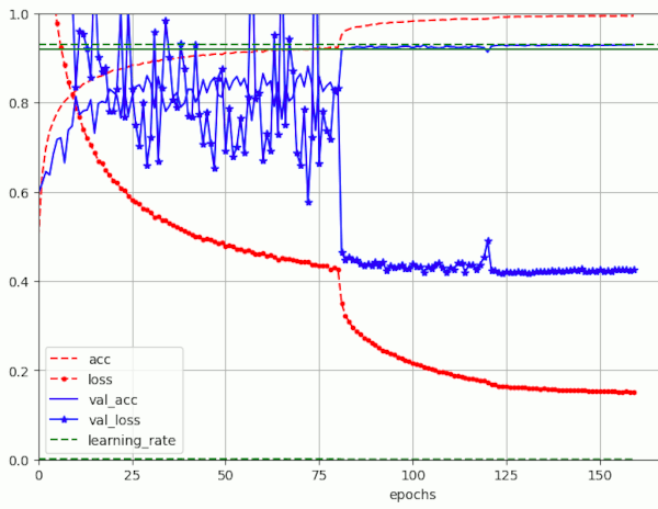
Results for a run with BS=128 (over 160 epochs) – reaching val_acc = 0.9306 (at epoch 130)

Note that the noise for the phase with a relatively high LR=0.001 has become even more pronounced than for BS=32. Whether we have to blame shuffling and/or ReduceLROnPlateau() for this remains to be seen. So far, we cannot confirm the quoted formula on the noise variation.

Observation 5: Accuracy values on the training set above 0.95 are required

To bring the validation accuracy above 0.92 typically accuracy values on the training data around and above acc=0.95 are required. So, if we want to bring down the required number of epochs from above 80 we also must reach high accuracy values during training pretty soon.

Convergence? Earlier?

We should be aware of the fact that the convergence of a ML model depends on the fulfillment of the following assumption:

During training we will sooner or later reach a region on the loss hyper-surfaces for both the training and the validation data where we move along the bottom a relatively broad valley compared to the Learning Rate and weight changes. Such that the walls of the loss hyper-surface along this valley appear remote for both the training and the validation data sets.

The image for BS=32 above indicates that we have reached such a valley latest at epoch 80. When we reduce the LR then by a factor of 10 the noise is drastically damped an convergence to a minimum of the loss takes also place for the validation samples. So, we end up with the following questions:

Do we need to care about the noise regarding our path on the loss hyper-surface for the validation samples?
How fast could we cross the region on the hyper-surface where the gradients are changing rapidly? Could we replace the initial LR=1.e-3 by another value which provide a faster convergence?
Could we reduce the Leaning Rate in a more continuous way?
At which epoch can we reduce the Learning Rate – without missing the valley which contains a hopefully global minimum?
Is the initial “noise” good noise in the sense that it helps to find a global minimum?

We have to find answers step by step with the help of further experiments.

Conclusion

The handling of a ResNet56v2 models as described by R. Atienza provides high validation accuracy values in the range between 0.92 and 0.93. Such values depend on the batch size (amongst other things), but can be reproduced with some variation in the required epoch number. Higher batch sizes appear to be preferable if you want to reach these values as early as possible.

However, even in the best case the LR-scheduler proclaimed by Atienza requires at least 82 epochs to get over a validation accuracy value of 0.91 and above 83 epochs to reach a validation accuracy of 0.92. We should first test if one can reduce the Learning Rate earlier with Atienza’s piecewise constant LR-scheduler. But, it also seems to be a good idea to program and test a LR-scheduler which reduces the Learning Rate in a more continuous fashion. An alternative for reaching a high accuracy level earlier could be to move to another optimizer.

All of these methods will be investigated in the forthcoming posts of this mini-series. For a study on a piecewise linear LR schedule see the next post:

AdamW for a ResNet56v2 – II – linear LR-schedules, Adam, L2-regularization, weight decay and a reduction of training epochs