In the 1st post of this series
ResNet basics – I – problems of standard CNNs
I gave an overview over building blocks of standard Convolutional Neural Networks [CNN]. I also briefly discussed some problems that come up when we try to build really deep networks with multiple stacks of convolutional layers [e.g. Conv1D- or Conv2D-layers of the Keras framework].
In this 2nd post I discuss the core elements of so called deep Residual Networks [ResNets]. ResNets have been published in multiple versions. The versions differ by the structure of so called Residual Units [RUs], which can be regarded as elementary bricks of a ResNet architecture. A RU can have a complex inner structure composed of basic layers as Conv2D-, Activation and Normalization-layers.
I only cover basic elements of the ResNet V2 architecture. I will do this in a personal introductory and summarizing way. The original research papers of He, Zhang, Ren and Sun (see [1] to [3]) will give you much more details and information. Concerning a solid approach to programming ResNets with the help of Keras and Tensorflow 2 you will find more information in [4] and in future posts of this blog. I strongly recommend to have a look at the named literature.
Level of this post. Advanced. You should be familiar with CNNs both theoretically and regarding numerical experiments.
Changes, 01/12/2024: Some drawings were changed to correct wrong layer-indices
Basic idea: Transfer of unfiltered data in parallel to filtering
At the end of the previous post I have pointed out that an inner Conv2D-layer of a standard CNN adapts its filters to already filtered data coming from previous layers. Thus the knowledge stored in the Conv2D-maps is build on filters of previous layers. Consequences are:
- An inner Conv2D-layer of a CNN cannot learn something from original input information.
- All of a CNN’s layers must together, i.e. as a unit, find an optimal solution of their combined filters during training.
How could an extended approach look like? How could filters of an inner group of layers adapt to unfiltered data? At least partially? Your spontaneous answer will probably suggest the following:
To enable a partial adaption of layers to unfiltered data one must somehow enable a propagation of unfiltered information throughout the network.
One of the basic ideas of ResNets is that the filters of a group of convolutional layers should adapt to patterns in the difference of its last map’s output in comparison to the input data presented to the group. I.e. the maps of such a filtering group should, during training, adapt to relevant patterns in the difference of filtered (=convoluted) data minus the original input data. (“Relevant” means important for solving a defined task as e.g. classification.) For the information transport between filtering units this means that we must actually propagate tensors of filtered data plus a tensor of original data. For some math see the next post in this series.
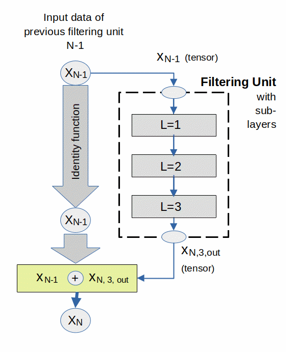
Thus we can make our simple answer consistent with a basic ResNet idea by adding original input tensors to the output of basic filtering units. Transporting original tensors alongside a filtering unit means that these tensors must be mapped to a new location by a simple identity function.
For the purpose of illustration let us assume that we have a group of sequential Conv2D-layers (L=1,2,3). We regard this group as a filtering unit. Then our idea means that we must add the original input tensor to the unit’s output tensor before we transfer the sum as input to the next filtering unit.

Residual Units and Residual Layers
To use the ResNet vocabulary we say that our group Conv2D-layers forms a “Residual Unit” [RU]. (“Residual” refers to the difference with results of an identity transformation.) Residual Units in turn can be stacked to form larger entities (Residual Stacks [RS]) of a ResNet-architecture; see below. Some people use the word Stages instead of stacks.
Inside a RU we may typically find an arrangement of some sub-layers, so called Residual Layers [RLs]. In a ResNet V2 we find just an ordered sequence of RLs with different properties. An RL can itself have a complex sub-structure comprising an arrangement of standard layers which apply convolutional, normalization and activation operations. I will come back to this substructure for ResNet V2 in a separate section below.
Stacks of Residual Units
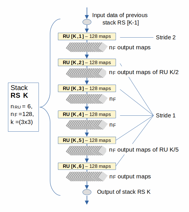
How would we get a well-defined stack of RUs? We would not vary all properties of the comprised RUs wildly. In principle a new stack in a ResNet most often comes with a new level of resolution. But within a stack the resolution of the output– maps of each RU is kept constant. For reasons of simplicity we request the following:
Both the number of filters and the dimensions of the output-maps of all RUs in a well defined Stack RS (of a ResNet V2) do not change.
You have to be careful here: We only refer to the number and dimensions of output-maps of the RUs. We will see later that both the dimension of filters and as well the number of filters and maps can change from RL to RL within a RU. In addition at the 1st RL within the very first RUs of a stack the stride changes.
But within a stack of RUs we neither change the number nF of output filters/maps of the RUs, nor the dimensions of the output-maps of the last Conv2D-layer (RL) in each RU. Actually, we use these properties as part of the definition of a residual stack collecting the same type of RUs.
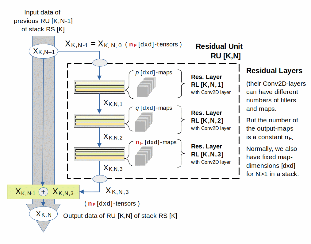
The following images shows this principle for the information flow within one stack RS and then for one RU within a defined stack :

In the example I indicated a (3×3) kernel. Regarding the change of the stride see below.

In the drawing above the transport of original information is shown as a (gray) side-track on the left. A potential sub-structure of different standard layers in a RL is indicated by varying colors. The maps belong to a Conv2D-layer (light orange) of each RL. The maps of the last RL are the output-maps of the RU.
Despite changing kernel-dimensions used for the Conv2D-layers in the different RLs the respective dimensions of the resulting maps inside a RU can be kept constant via setting padding = “same”. So, the dimensions of the maps remain constant for all RUs/RLs of a certain stack (with the exception of the RU’s first RL; see below).
Regarding the number of maps p, q, nF: Referring to the drawing we typically can use p = nF / 2, q = p (see [4] and below). But also a reductions in map-depth p = nF / 4 have been used. For respective kernel dimensions and other details see a section on the RL-sub-structure for ResNet V2 networks below.
A really important point in the drawing for a RU is that the RU’s output is a pure superposition of the original signal with filtered data. Thus the original data can propagate through the whole net during the training phase of a ResNet V2. As the weights in the filtering part typically remain small for a while after initialization, all layers will initially have a chance to adapt their filters to the original input information. But also in later phases of the training the original information can spread itself as a major contribution to the input of all RUs in a RS stack.
The next plot condenses the information transport a bit by placing the transfer path of the original data inside a Residual Unit. This kind of presentation does not give us any more information, but is a bit more helpful for a later programming of RUs with the help of Keras (or PyTorch).

We speak of a “Shortcut Connection” or “Skip Connection” regarding the transfer of the original information: It bridges the sequence of RL-sublayers of a RU. Such a RU is regarded a kind of basic unit for information processing in ResNets.
Regarding the difference of ResNet V1 vs. ResNet V2:
The plain addition of the signals at the output-side of a RU came with version V2 of ResNets in [2]. It marked a major difference in comparison to [1] and ResNet V1 architectures. In contrast to previous architectures, in a ResNet V2 architecture we do not apply an activation function to the sum at the output side of a RU. This enables a propagation of unfiltered data throughout the whole net.
Resolution reduction and special shortcut connections in the 1st RU of a stack
Also ResNets must realize a basic principle of CNNs: Patterns should be detected on different length scales or spatial dimensions. I.e., we need stacks of RUs and RLs working on averaged data of lower resolution.
In CNNs we mark a point of a transition to lower resolution either by a pooling layer or by a convolutional layer with a stride s > 1, e.g. s = 2. In a ResNet V2 we use special RUs that contain a first RL (and related Conv2D) having a stride s = 2. Such a RU appears as the 1st RU of a new stack of RUs working on a lower resolution level, i.e. with maps of smaller dimensions.
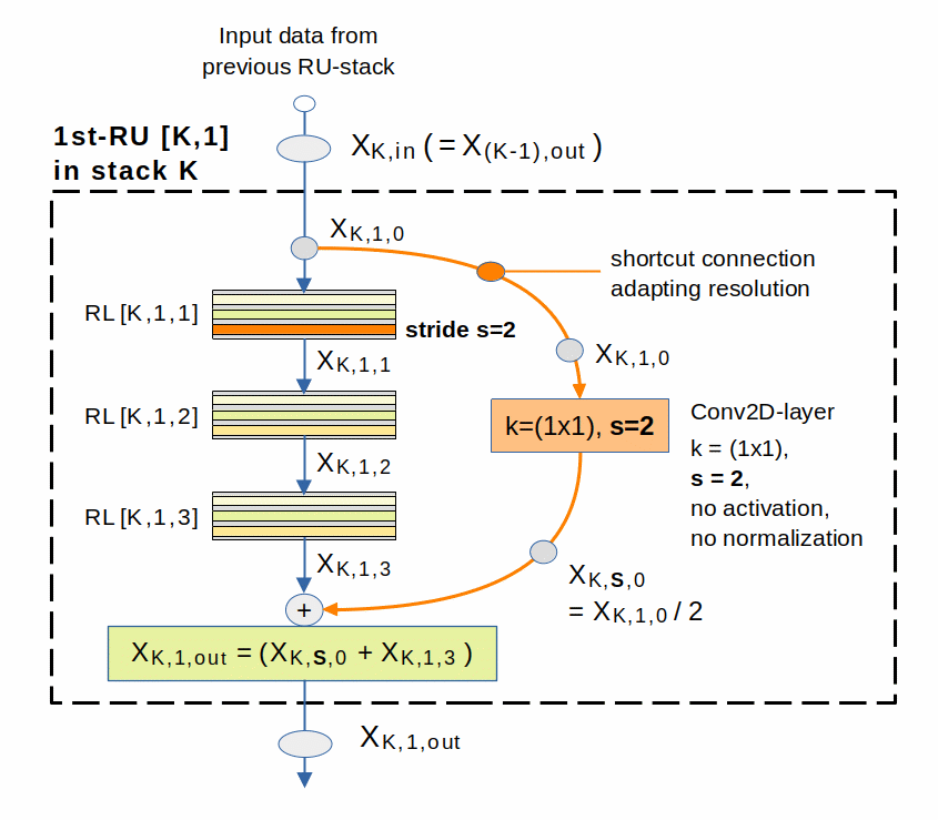
The drawings above make it clear that such a (1st) RU [K/1] of a stack RS [K] must do something special along its shortcut-connection to keep the resolution of the transported unfiltered input data aligned with the filtered output of the RU’s output-maps.
The most simple way to achieve equal dimensions of the tensors is to employ a Conv2D-layer with equal stride s = 2 along the shortcut. Such a special shortcut-connection is shown in the next graphics:

There is a consequence of this pattern which we cannot avoid:
The original image information is not propagated unchanged throughout the whole ResNet. Instead lower resolution variants of the original input data are propagated as contributions through the RUs of each stack.
Exception to the rule that the stride has a value of 2 in the shortcut layer:
In the very first first stack we have stride=1.
Architectural Hierarchy – Stacks of RUs, Residual Units, Residual Layers, Sub-Layers
Putting the elements discussed above together we arrive at the following architectural hierarchy of a deep ResNet V2:
- A first Conv2D-layer that initially scans the Input data by a filter of suitable dimensions. The Conv2D-layer is accompanied by some standard sub-layers as a Input- a BatchNormalization-, Activation- and sometimes by an additional second Conv2D-Layer reducing resolution.
- Stacks of Residual Units with the same number of convolutional filters nF. nF varies from stack to stack. All maps of convolutional layers within a stack shall have the same resolution.
- Residual Unit [RU] (comprising a fixed number of so called Residual Layers)
- Residual Layer [RL] (comprising some standard sub-layers; the sub-structure of RLs can vary between architecture versions)
- Standard Sub-Layers of a RL – including BatchNormalization-, Activation- and Conv2D-Layers in a certain order
- A classifying MLP-like network of fully-connected [FC] layers (classification) or a specific dense FC-layer to fill a latent space (Encoders).
The first layers filter, normalize, transform and sometimes average input data (training data) to an intermediate target resolution. Afterward we have multiple stacks of Residual Units [RUs], each with a shortcut connection. The depth of a network, i.e. the number of analyzing Conv2D– or Dense-layers depends mainly on the number of RUs in the distinguished stacks.
An example of a relatively simple ResNet V2 network could, on the level of RUs, look like this:

This example comprises 4 stacks of RUs (distinguished by different colors in the drawing). All RUs within a stack have a (fixed) number of RLs (not displayed). The number of RUs changes from nRU = 3 for RS1 to nRU = 6 for RS 2, nRU = 6 for RS 3 and eventually to nRU = 3 for RS 4. Each RL comprises a Conv2D-layer (not displayed above). Within the stack the Conv2D-output-layers of the RUs all have the same number of filters nF and of respective maps (64, 128, 256, 512).
As usual we raise the number of maps with shrinking resolution. All output maps of the RUs in a certain stack have the same dimensions. The central filter-kernel in the example is chosen to be k=(3×3) throughout all stacks, RUs and RLs (for the meaning of “central” see the section on a RL’s sub-structure below).
The blue curved lines symbolize the RUs’ shortcut connections. The orange lines instead symbolize special shortcut connections with an extra Conv2D-Layer with kernel (1×1) and stride=2. As discussed above, these special shortcuts compensate for the reduction of resolution and map-dimensions.
Note: The first stack RS1 does NOT change the Conv2D resolution; but it raises the number of filters.
Again: The advantage of such a structure is that inner layers can already start learning even if the filter-values in the “residual parts” of the first layers are still small.
Bottleneck Residual Units – and the sub-structure of their Residual Layers
A RU consists of Residual Layers [RLs]. Each RL in turn consists of a sequence of standard layers. The authors of [2] and [3] have investigated the effects of a big variety of different RU/RL sub-structures on convergence during training and on the error-rate of classification ResNets after training. The eventual optimal sub-structure of a RU (for ResNet V2) can be described as follows:
- A RU (of a ResNet V2) consists of 3 sub-layers, i.e. RLs (Residual Layers) in our terminology.
- Each of these Residual Layers comprises three standard sub-layers in the following sequential order
BatchNormalization Layer => Activation Layer (with the Relu function) => Conv2D Layer.
The only exception is the first RL of the the first stack (see below). - The number of output-maps is nF defined for the stack
- The 1st RL uses a Conv2D-layer with a (1×1)-kernel, a stride s=1 (s=2, only for the first RL of the first RU in a RU- stack), padding = “same”. The number of maps (depth) of this layer is reduced to nF/2 or nF/4.
- The 2nd RL uses a Conv2D-layer with a (3×3)-kernel, a stride s=1, padding=”same”. The number of maps (depth) of this layer is reduced to nF/2 or nF/4.
- The 3rd RL uses a Conv2D-layer with a (1×1)-kernel, a stride s=1, padding=”same”. The number of maps is nF.
“Optimal” refers to number of parameters, complexity and the level of accuracy. This structure is called a “botteneck“-architecture with full pre-activation. See the graphics below:

The term “pre-activation” is used because the activation occurs ahead of the convolution. Which is a remarkable deviation from previously used “wisdom” of performing activation after convolution.
The term “bottleneck” itself refers to a reduction of the number of maps used in the Conv2D-layers in RL [K,N,1] and RL[K,N,2] within the RL-sequence:
The first RL with k=(1×1) reduces the number of maps, i.e. the Conv2D-layer’s depth, by some factor (< 1) of the target number for output-maps nF for all RUs of the stack. The 2nd RL also works with this reduced number of maps. The 3rd RL, however, restores the number of maps to the target number nF.
Keep in mind when programming:
The depth-reduction of a bottleneck structure of RUs refers to the number of maps, not to the dimensions of the kernel and neither to the dimensions of the maps. This is often misunderstood.
Why do we perform such an intermittent depth-reduction of the Conv2D-layers at all? Well, an important argument is efficiency: We want to keep the number of weights, i.e. connections between the maps of different layers, as small as possible. I think the approach of R. Atienza in [4] to use a reduction factor 1/2, i.e. q = 1/2 * nF, is a very reasonable one as this is just the number of the previous stack.
First layers of a ResNet V2
We must work with the input data before we feed them into the first stack of Residual Units and split the data flow into a regular path through the sub-layers of RUs and residual shortcut connections. Reasons to prepare the data are:
- We may want to reduce resolution and dimensions to some target values.
- We may want to normalize the data.
- We may want to apply a first activation to get positive weights.
The handling depends both on the exact requirements for an adaption of the resolution of the images and efficiency conditions. Regarding a concrete approach the original research papers [1] to [3] show a tendency
- to first use a convolutional layer with a (3×3) or (7×7) kernel,
- to apply apply BatchNormalization afterward
- and perform a first activation (with Relu).
In this order. This has a consequence for the very 1st RL in 1st RU of the 1st stack: We can just omit the usual Activation- and BatchNormalization-Layers there. This kind of approach seems to support convergence and generalization during network training.
Different architectures and number of stacks/stages for the analysis of concrete objects
Regarding the number of stacks, the number of filters per stack and the number of RUs per stack, the papers [1] to [3] leave the reader a bit confused after a first reading. The authors obviously preferred different setups for different kinds of image classes – as e.g. for the ImageNet-, the CIFAR10- and the CIFAR100- and the MS COCO-datasets.
The original strategy in [1] for CIFAR10/100 classification tasks was to use a plain structure of 3 stacks, each with an equal number nRU of up to 18 RUs per stack and numbers of feature maps nF ∈ {16, 32, 64). For nRU = 9 this results in a ResNetV2-56 with 56 layers, for nRU = 18 in a ResNetV2-164, with 164 layers respectively. R. Atienza in [4] uses filter numbers nRU ∈ {64, 128, 256}. I find it also interesting that R. Atienza did not try out a different setup with 4 stacks for CIFAR10.
For more complex images other strategies may be more helpful. Geron in his book [5] discusses a setup of 4 stacks for the ImageNet dataset with the number of filters as {64, 128, 256, 512}, but with numbers of RUs as nRU ∈ {3, 4, 6, 3} for a ReNet-34.
This all means: We should prepare our codes to be flexible enough to cover up to four or five stacks with different numbers of RUs.
As we as private enthusiasts have very limited HW-resources, we can only afford to train a deep ResNet V2 on modest data sets like CIFAR10, Fashion MNIST, CelebA. Still, we need to experiment a bit. I particular we should investigate some time in finding out what depth reduction is possible in the bottleneck layers.
An open question
Personally, the study of [1] to [4] left me with an open question:
Why not additionally bridge a whole stack of RUs with a shortcut connection?
This would be an intermediate step in the direction of “Densely Connected Convolutional” networks [DenseNets]. Maybe this is an overkill, but let us keep this as an idea to investigate further.
Conclusion
ResNet V2 networks are somewhat more complex than standard CNNs. However, the recipes given in [1] to [4] are rather clear. Changing the number of stacks, the number of RUs in the stacks and the parameters of the Residual Bottleneck-Layers leaves more than enough room for experiments and adaptions to specific input data sets. We just have to implement respective parameters and controls in our Python programs. In the next post of this series I will look at bit at the mathematical analysis for a sequence of RUs.
Literature
[1] K. He, X. Zhang, S. Ren , J. Sun, “Deep Residual Learning for Image Recognition”, 2015, arXiv:1512.03385v1
[2] K. He, X. Zhang, S. Ren , J. Sun, “Identity Mappings in Deep Residual Networks”, 2016, version 2 arXiv:1603.05027v2
[3] K. He, X. Zhang, S. Ren , J. Sun, “Identity Mappings in Deep Residual Networks”, 2016, version 3, arXiv:1603.05027v3
[4] R. Atienza, “Avanced Deep Learning with Tensorflow 2 and Keras”, 2nd edition, 202, Packt Publishing Ltd., Birmingham, UK (see chapter 2)
[5] F. Chollet, “Deep Learning with Python”, 2017, Manning Publications, USA
[6] A. Geron, “Hands-On Machine Learning with Scikit-Learn, Keras & TensorFlow”, 3rd ed., 2023, O’ReillyMedia Inc., Sebastopol, USA CA