Convolutional Neural Networks [CNNs] do a good job regarding the analysis of image or video data. They extract correlation patterns hidden in the numeric data of our media objects, e.g. images or videos. Thereby, they get an indirect access to (visual) properties of displayed physical objects – like e.g. industry tools, vehicles, human faces, ….
But there are also problems with standard CNNs. They have a tendency to eliminate some small scale patterns. Visually this leads to smoothing or smear-out effects. Due to an interference of applied filters artificial patterns can appear when CNN-based Autoencoders shall recreate or generate images after training. In addition: The number of sequential layers we can use within a CNN on a certain level of resolution is limited. This is on the one hand due to the number of parameters which rises quickly with the number of layers. On the other hand and equally important vanishing gradients can occur during error-back-propagation and cause convergence problems for the usually applied gradient descent method during training.
A significant improvement came with so called Deep Residual Neural Networks [ResNets). In this post series I discuss the most important differences in comparison to standard CNNs. I start the series with a short presentation of some important elements of CNNs. In a second post I will directly turn to the structure of the so called ResNet V2-architecture [2].
To get a more consistent overview over the historical development I recommend to read the series of original papers [1], [2], [3] and a chapter in the book of R. Atienza [4] in addition. This post series only summarizes and comments the ideas in the named resources in a rather personal way. For me it serves as a preparation and overall documentation for Python programs. But I hope the posts will help some other readers to start working with ResNets, too. In a third post I will also look at the math discussed in some of the named papers on ResNets.
Level of this post: Advanced. You should be familiar with the concepts of CNNs and have some practical experience with this type of Artificial Neural Network. You should also be familiar with the Keras framework and standard layer-classes provided by this framework.
Elements of simple CNNs
A short repetition of a CNN’s core elements will later help us to better understand some important properties of ResNets. ResNets are in my opinion a natural extensions to CNNs and will allow us to build really deep networks based on convolutional layers. The discussion in this post focuses on simple standard CNNs for image analysis. Note however, that the application spectrum is much broader, 1D-CNNs can for example be used to detect patterns in sequential data flows as texts.
We can use CNNs to detect patterns in images that depict objects belonging to certain object-classes. Objects of a class have some common properties. For real world tasks the spectrum of classes must of course be limited.
The idea is that there are detectable patterns which are characteristic of the object classes. Some people speak of characteristic features. Then the identification of such patterns or features would help to classify objects on a new images a trained CNN gets confronted with. Or a combination of patterns could help to recreate realistic object images. A CNN must therefore provide not only some mechanism to detect patterns, but also a mechanism for an internal pattern representation which can e.g. be used as basic information for a classification task.
We can safely assume that the patterns for objects of a certain class will show specific structures on different length scales. To cover a reasonable set of length scales we need to look at images at different levels of resolution. This is one task which a CNN must solve; certain elements of its layer architecture must ensure a systematic change in resolution and of the 2-dimensional length scales we look at.
Pattern detection itself is done by applying filters on sub-scales of the spatial dimensions covered by a certain level of resolution. The filtering is done by so called “Convolutional Layers“. A filter tests the overlap of a given object’s 2-diimensional structures with some filter-related periodic pattern on smaller scales. Relevant filter-parameters for optimal patterns are determined during the training of a CNN. The word “optimal” refers to the task the CNN shall eventually solve.
The basic structure of a CNN (e.g. to analyze the MNIST dataset) looks like this:
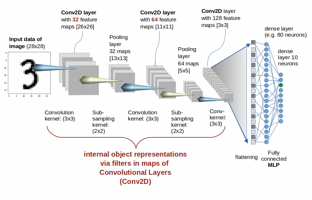
The sketched simple CNN consists of only three “Convolutional Layers”. Technically, the Keras framework provides a convolutional layer suited for 2-dimensional tensor data by a Python class “Conv2D“. I use this term below to indicate convolutional layers.
Each of our CNN’s Conv2D-layers comprises a series of rectangular arrays of artificial neurons. These arrays are called “maps” or sometimes also “feature maps“.
All maps of a Conv2D-layer have the same dimensions. The output signals of the neurons in a map together represent a filtered view on the original image data. The deeper a Conv2D-layer resides inside the CNN’s network the more filters had an impact on the input and output signals of the layer’s maps. (More precisely: of the neurons of the layer’s maps).
Resolution reduction (i.e. a shift to larger length scales) is in the depicted CNN explicitly done by intermittent pooling-layers. (An alternative would be that the Conv2D-layers themselves work with a stride parameter s = 2; see below.) The output of the innermost convolution layer is flattened into a 1-diemsnional array, which then is analyzed by some suitable sub-network (e.g. a tiny MLP).
Filters and kernels
Convolution in general corresponds to applying a (sub-scale) filter-function to another function. Mathematically we describe this by so called convolution integrals of the functions’ product (with a certain way of linking their arguments). A convolution integral measures the degree of overlap of a (multidimensional) function with a (multidimensional) filter-function. See here for an illustration.
As we are working with signals of distinct artificial neurons our filters must be applied to arrays of discrete signal values. The relevant arrays our filters work upon are the neural maps of a (previous) Conv2D-layer. A sub-scale filter operates sequentially on coherent and fitting sub-arrays of neurons of such a map. It defines an averaged signal of such a sub-array which is fed into a neuron of map located in the following Conv2D-layer. By sub-scale filtering I mean that the dimensions of the filter-array are significantly smaller than the dimensions of the tested map. See the illustration of these points below.
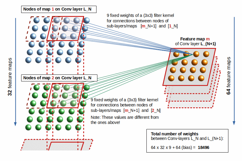
The sub-scale filter of a Conv2D-layer is technically realized by an array of fixed parameter-values, a so called kernel. A filter’s kernel parameters determine how the signals of the neurons located in a covered sub-array of a map are to be modified before adding them up and feeding them into a target neuron. The parameters of a kernel are also called a filter’s weights.
Geometrically you can imagine the kernel as an (k x k)-array systematically moved across an array of [n x n]-neurons of a map (with n > k). The kernel’s convolution operation consists of multiplying each filter-parameter with the signal of the underlying neuron and afterward adding the results up. See the illustration below.
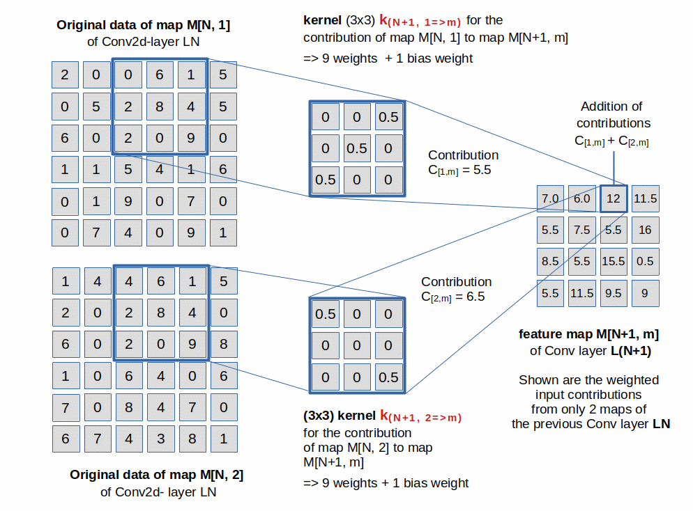
For each combination of a map M[N, i] of a layer LN with a map M[N+1, m] of the next layer L(N+1) there exists a specific kernel, which sequentially tests fitting sub-arrays of map M[N, i] . The filter is moved across map M[N, i] with a constant shift-distance called stride [s]. When the end of a row is reached the filter-array is moved vertically down to another row at distance s.
Note on the difference of kernel and map dimensions: The illustration shows that we have to distinguish between the dimensions of the kernel and the dimensions of the resulting maps. Throughout this post series we will denote kernel dimensions in round brackets, e.g. (5×5), while we refer to map dimensions with numbers in box brackets, e.g. [11×11].
In the image above map M[N, i] has a dimension of [6×6]. The filter is based on a (3×3) kernel-array. The target maps M[N+1, m] all have a dimension of [4×4], corresponding to a stride s=1 (and padding=”valid” as the kernel-array fits 4 times into the map). For details of strides and paddings please see [5] and [6].
Whilst moving with its assigned stride across a map M[N, i] the filter’s “kernel” mathematically invokes a (discrete) convolutional operation at each step. The resulting number is added to the results of other filters working on other maps M[N, j]. The sum is fed into a specific neuron of a target map M[N+1, m] (see the illustration above).
Thus, the output of a Conv2D-layer’s map is the result of filtered input coming from previous maps. The strength of the remaining average signal of a map indicates whether the input is consistent with a distinct pattern in the original input data. After having passed all previous filters up to the length scale of the innermost Conv2D-layer each map reacts selectively and strongly to a specific pattern, which can be rather complex (see pattern examples below).
Note that a filter is not something fixed a priori. Instead the weights of the filters (convolution kernels) are determined during a CNN’s training and weight optimization. Loss optimization dictates which filter weights are established during training and later used at inference, i.e. for the analysis of new images.
Note also that a filter (or its mathematical kernel) represents a repetitive sub-scale pattern. This leads to the fact that patterns detected on a specific length scale very often show a certain translation and a limited rotation invariance. This in turn is a basic requirement for a good generalization of a CNN-based algorithm.
A filter feeds neurons located in a map of a following Conv2D-layer. If a layer N has p maps and the following layer has q maps, then a neuron of a map M[N+1, m] receives the superposition of the outcome of (p*q) different filters (and respective kernels).
Patterns and features
Patterns which fit some filters, of course appear on different length scales and thus at all Conv2D-layers. We first filter for small scale patterns, then for (overlayed) patterns on larger scales. A certain combination of patterns on all length scales investigated so far is represented by the output of the innermost maps.
All in all the neural activation of the maps at the innermost layers result from (surviving) signals which have passed a sequence of non-linearly interacting filters. (Non-linear due to the non-linearity of the neurons’ activation function.) A strong overall activation of an innermost map corresponds to a unique and characteristic pattern in the input image which “survived” the chain of filters on all investigated scales.
Therefore a map is sometimes also called a “feature map”. A feature refers to a distinct (and maybe not directly visible) pattern in the input image data to which an inner map reacts strongly.
Increasing number of maps with lower resolution
When reducing the length scales we typically open up space for more significant pattern combinations; the number of maps increases with each Conv-layer (with a stride s=2 or after a pooling layer). This is a very natural procedure due to filter combinatorics.
Examples of patterns detected for MNIST images
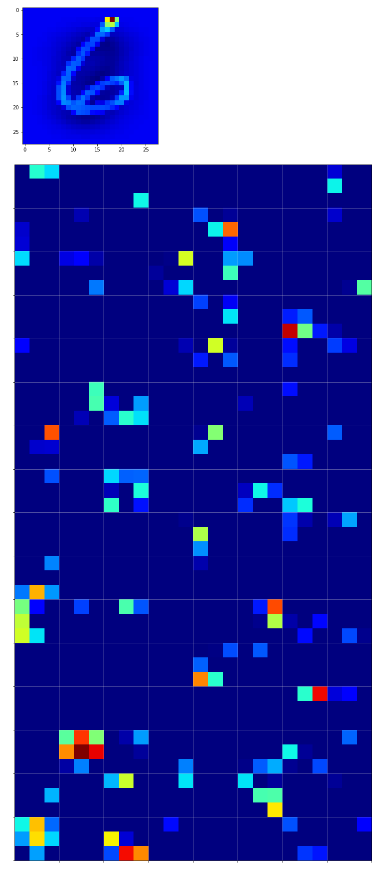
A CNN in the end detects and establishes patterns (inherent in the image data) which are relevant for solving a certain problem (e.g. classification or generative reconstruction). A funny thing is that these “feature patterns” can be visualized.
The next image shows the activation pattern (signal strengths) of the neurons of the 128 (3×3) innermost maps of a CNN that had been trained for the MNIST data and was confronted with an image displaying the digit “6”.
The other image shows some “featured” patterns to which six selected innermost maps react very sensitively and with a large averaged output after having been a trained on MNIST digit images.
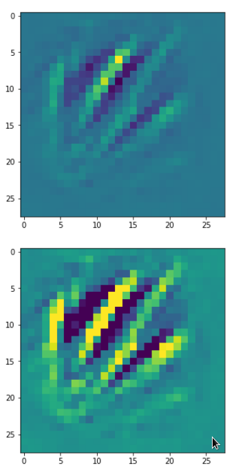
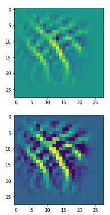
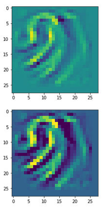
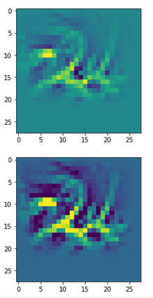
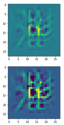
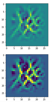
These patterns obviously result from translations and some rotation of more elementary patterns. The third pattern seems to useful for detecting “9”s at different positions on an image. The fourth pattern for the detection of images of “2”s. It is somewhat amusing of what kind of patterns a CNN thinks to be interesting to distinguish between digits!
If you are interested of how to create images of patterns to which the maps of the innermost Conv2D-layer reacts to see the book of F. Chollet on “Deep Learning with Python” [5]. See also a post of the physicist F. Graetz “How to visualize convolutional features in 40 lines of code” at “towardsdatascience.com”. For MNIST see my own posts on the visualization of filter specific patterns in my linux-blog. I intend to describe and apply the required methods for layers of ResNets somewhere else in the present ML-blog.
Deep CNNs
The CNN depicted above is very elementary and not a really deep network. Anyone who has experimented with CNNs will probably have tried to use groups of Conv2D-layers on the same level of resolution and map-dimensions. And he/she probably will also have tried to stack such groups to get deeper networks. VGG-Net (see the literature, e.g. [2, 5, 6] ) is a typical example of a deeper architecture. In a VGG-Net we have a group of sequential Conv2D layers on each level of resolution – each with the same amount of maps.
BUT: Such simple deep networks do not always give good results regarding both error rates, convergence and computational time. The number of parameters rises quickly without a really satisfactory reward.
Problems of deep CNNs
In a standard CNN each inner convolutional layer works with data that were already filtered and modified by previous layers.
An inner filter can not adapt to original data, but only to filtered information. But any filter does eliminate some originally present information … This also occurs at transitions to layers working on larger dimensions, i.e. with maps of reduced resolution: The first filter working on a larger length scale (lower resolution) eliminates information which originally came from a pooling layer (or a Conv2D-layer with stride=2). The original averaged data are not available to further layers working on the same new length scale.
Therefore, a standard CNN deals with a problem of rather fast information reduction. Furthermore, the maps in a group have no common point of reference – except overall loss optimization. Each filter can eventually only become an optimal one if the previous filtering layer has already found a reasonable solution. An individual layer cannot learn something by itself. This in turn means: During training the net must adapt as a whole, i.e. as a unit. This strong coupling of all layers can enhance the number of training epochs and also create problems of convergence.
How could we work against these trends? Can we somehow support an adaption of each layer to unfiltered data – i.e. support some learning which does not completely dependent on previous layers? This is the topic of the next post in this series.
Conclusion
CNNs were building blocks in the history of Machine Learning for image analysis. Their basic elements as Conv2D-layers, filters and respective neural maps on different length scales (or resolutions) work well in networks whose depth is limited, i.e. when the total number of Conv2D-layers is small (3 to 10). The number of parameters rises quickly with a network’s depth and one encounters convergence problems. Experience shows that building really deep networks with Conv2D-layers requires additional architectural elements and layer-combinations. Such elements are cornerstones of Residual Networks. I will discuss them in the next post of this series. See
ResNet basics – II – ResNet V2 architecture
Literature
[1] K. He, X. Zhang, S. Ren , J. Sun, “Deep Residual Learning for Image Recognition”, 2015, arXiv:1512.03385v1
[2] K. He, X. Zhang, S. Ren , J. Sun, “Identity Mappings in Deep Residual Networks”, 2016, version 2 arXiv:1603.05027v2
[3] K. He, X. Zhang, S. Ren , J. Sun, “Identity Mappings in Deep Residual Networks”, 2016, version 3, arXiv:1603.05027v3
[4] R. Atienza, “Avanced Deep Learning with Tensorflow 2 and Keras”, 2nd edition, 202, Packt Publishing Ltd., Birmingham, UK (see chapter 2)
[5] F. Chollet, “Deep Learning with Python”, 2017, Manning Publications, USA
[6] A. Geron, “Hands-On Machine Learning with Scikit-Learn, Keras & TensorFlow”, 3rd ed., 2023, O’ReillyMedia Inc., Sebastopol, USA CA