In this post series we try to find methods to reduce the number of epochs for the training of ResNets on image datasets. Our test case is CIFAR10. In this post we will test a modified cosine shaped schedule for a systematic and fast reduction of the learning rate LR. This supplements the approaches described in previous posts of this series
- AdamW for a ResNet56v2 – II – linear LR-schedules, Adam, L2-regularization, weight decay and a reduction of training epochs
- AdamW for a ResNet56v2 – III – excursion: weight decay vs. L2 regularization in Adam and AdamW ,
- AdamW for a ResNet56v2 – IV – better accuracy and shorter training by pure weight decay and large scale fluctuations of the validation loss .
So far we have studied piecewise linear decay schedules for the Learning Rate [LR] in combination with pure Weight Decay [WD]. We shall first review the results achieved so far and the methods used. Afterward we will perform further numerical experiments during which the LR reduction follows a cosine curve between 0 and π/2.
We will see that we can bring the number of training epochs to reach our threshold value for the validation accuracy val_acc ≥ 0.92 down to 21. However, despite this seeming success, there are indications that we get stuck on the loss hyper-surface without having reached the bottom of the global minimum. This also sets some question mark behind 1Cycle approaches.
Success factors so far: Fluctuations and a substantial reduction of the weight decay ahead of a final training phase
Weight decay helps to regularize the network’s weight values. We have applied weight decay by using the Keras implementation of the AdamW optimizer and controlled the WD-strength by a parameter λ = 1/α * λwd. During the experiments we saw that relatively big λ-values (λ ≥ 0.1) triggered large scale fluctuations in the validation loss during certain training phases. These fluctuations were, however, helpful to raise the eventual validation accuracy val_acc. The following plots give an impression for a test run over 60 epochs:
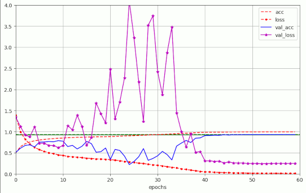
Note the very low value of the loss (red-dotted line) at the end of the final training phase (loss ≤ 0.016). We find no shift of the loss minimum to values significantly above the zero-line in our runs with pure WD. This is very different from runs with L2-regularization.
The accuracy for the training data approaches almost 100% (acc ≥ 0.99). This is an indication that these long runs really approach a global minimum.
We have interpreted the fluctuations as an effect triggered by a constant extra drift exerted by WD towards the origin of the multidimensional Euclidean coordinate system spanned by axes for the individual weight values of the ResNet. Meaning: WD permanently adds an extra vector (pointing to the origin) to the loss gradient – and thus forces the weights to change in a direction off the direction of the original loss gradient. The resulting reduction of the weights may have stronger consequences in the “val_loss”-hypersurface of the validation data than on the loss hyper-surface of the training data. In particular when we reach values with steep side walls.
Convergence between 30 and 35 epochs?
What about runs with fewer epochs? So far, we were able to bring the number of epochs for breaking our threshold values of val_acc = 0.92 and val_acc = 0.93 down to below 30 and 35 epochs, respectively. In comparison to an approach of Atienza in [1] this is already a reduction by around 70 to 90 epochs. We have not changed our general recipe for the LR schedule, yet:
We damped the weight decay [WD] (and the WD induced fluctuations) impact ahead of a final convergence phase of the training. We achieved this indirectly by a fast reduction of the learning rate LR, which also reduced the WD correction term by up to two orders of magnitude. α denotes the initial learning rate. λ the weight decay parameter provided to the AdamW optimizer in its Keras implementation. The experiments in the preceding post clearly showed that when the LR drops below a tenth of the initial LR α
the fluctuations in the validation loss are damped sufficiently enough, such that we can approach an undisturbed minimum of the training loss – and thus (hopefully) also of the validation loss.
The problem with this approach is that we depend on the reduction of the LR, only. The extreme reduction also almost stops the systems movement on the loss-hypersurface during the few remaining epochs. I will come back to this point later. For the time being I want you to note that we do not reach the extremely low loss’ minimum value we achieved in longer runs.
Cosine based schedules of the Learning Rate
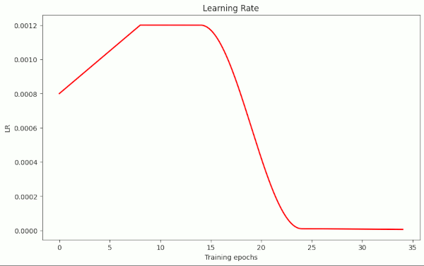
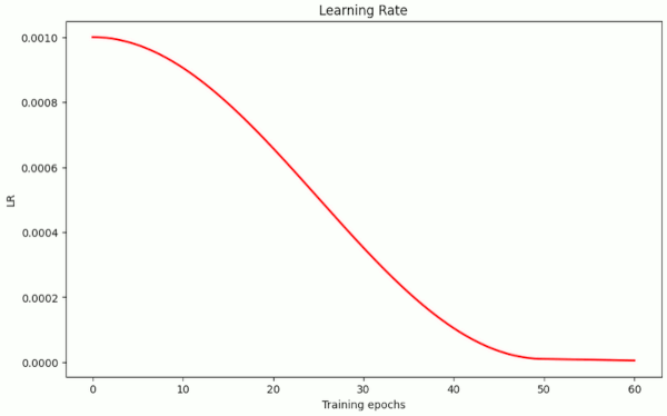
Let us see whether a cosine shaped LR schedule works equally well as a piecewise linear one. The advantage of a piecewise linear schedule was that we could define a relatively long initial phase with a high and constant value of the initial learning rate α. To compensate for this and to allow for a steep initial rise of the LR in the sense of 1Cycle-approaches I have modified the computation of LR during the training iterations, such that it allows for two preceding initial phases before the cosine based decay of the LR is applied. The last phase is also handled as a linear one. The plot below shows the general form of such a LR schedule.
Illustration 1: LR schedule with initial linear rise, a plateau and a cosine shaped decline of the LR
Let us now apply different variants of such a cosine based schedule.
Common properties of the runs
In the following experiments the validation data sets (comprising 10,000 samples) were individually created per run, but the selected samples were stratified according to the general distribution of images over the 10 categories of CIFAR10. The mini-batch size was chosen to be BS=64. Reasons for this choice were given in previous posts. The value of the LR after the cosine shaped decay typically were more than 2 orders of magnitude smaller than the initial LR-value α. The training samples were shuffled between the epochs of the training.
A smooth LR decay over 50 epochs
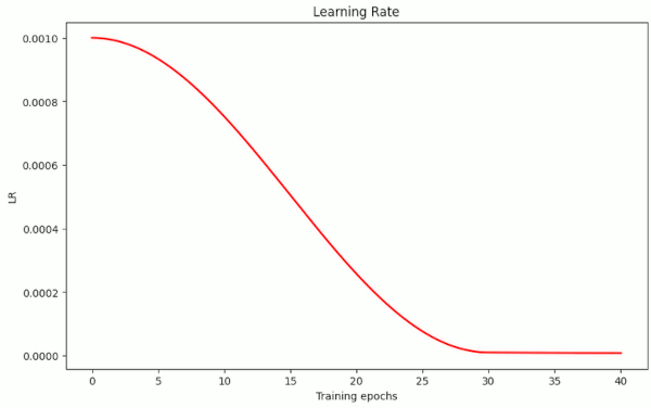
First I want to show that a continuous smooth LR decay over 50 epochs works – and that we get similar values as for the piecewise linear variation. The LR schedule looked like the one shown in illustration 2 below ( taken from run 5 in the table 1 below).
Illustration 2: LR schedule with a cosine shaped decline of the LR from epoch 0 onward
Between epochs 50 and 60 a linear LR reduction took place in some of the first runs. The batch size was BS=64 in all runs. Respective results were:
Table 1 – runs over 50 to 60 epochs
| # | epoch | acc_val | acc | epo best | val acc best | final loss | final val loss | shift | l2 | λ | α | LR reduction phases |
| 1 | 47 | 0.92420 | 0.9916 | 53 | 0.93000 | 0.0121 | 0.2701 | 0.07 | 0.0 | 0.094 | 1.e-3 | [1.e-3, 0]cos[0, 56] |
| 2 | 44 | 0.92240 | 0.9922 | 49 | 0.92560 | 0.0138 | 0.2750 | 0.07 | 0.0 | 0.100 | 1.e-3 | [1.e-3, 0]cos[0, 52] |
| 3 | 42 | 0.92100 | 0.9911 | 53 | 0.92690 | 0.0118 | 0.2695 | 0.07 | 0.0 | 0.100 | 1.e-3 | [1.e-3, 0]cos[1.e-5, 50]lin[2.e-6, 60] |
| 4 | 46 | 0.92260 | 0.9941 | 52 | 0.92830 | 0.0125 | 0.2687 | 0.07 | 0.0 | 0.140 | 1.e-3 | [1.e-3, 0]cos[1.e-5, 50]lin[5.e-6, 60] |
| 5 | 48 | 0.92470 | 0.9942 | 53 | 0.93260 | 0.0143 | 0.2451 | 0.07 | 0.0 | 0.200 | 1.e-3 | [1.e-3, 0]cos[1.e-5, 50]lin[5.e-6, 60] |
The meaning of the parameters given were explained in previous posts of this series. The brackets [LR-target value, epoch] give you the target value of the LR reached at a certain epoch. The abbreviations “lin” and “cos” before a bracket indicate the type of LR variation.
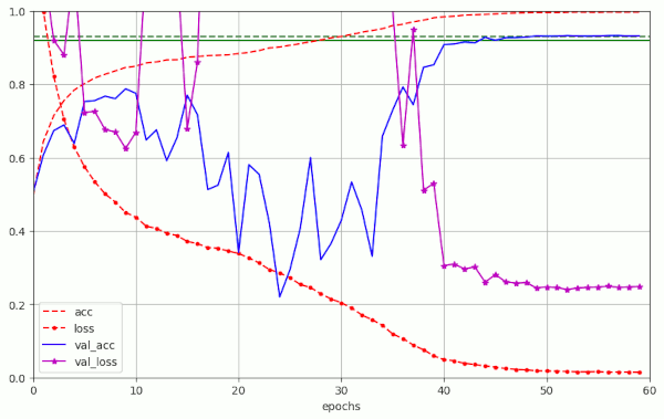
Plots for run 5 are given below:
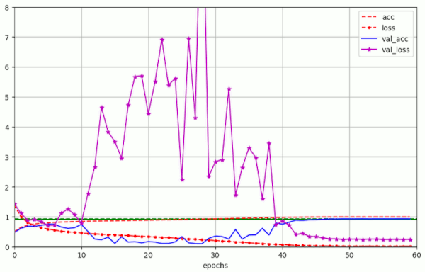
We again see the huge fluctuations in the validation loss (which could be specific for the CIFAR10 dataset). We also approach a very low final loss-value – similar to the values reached with piecewise linear schedules over 50 epochs.
A in the case of piecewise linear schedules, we see again that the shrinking of the LR and thereby also of the diminishing WD contribution to the weight correction eventually leads to the expected values of the validation accuracy. In run 5 we pass val_acc = 0.924 at epoch 48 and val_acc ≥ 0.93 at epoch 53. A relative high value of λ= 0.2 was required to achieve this result.
Reducing training and the LR cosine phase to around 30 epochs
The following table summarizes results for runs with a smaller number of epochs. All the runs started the cosine shaped reduction of LR directly from the first epoch on and thus were structurally very similar to the runs up to epochs 50 or 60 above. As we reduced the LR drastically we did not expect to reach the bottom of a global loss minimum – even if we reached the surroundings of such a minimum.
Table 2 – runs over 30 to 40 epochs
| # | epoch | acc_val | acc | epo best | val acc best | final loss | final val loss | shift | l2 | λ | α | LR reduction phases |
| 6 | 28 | 0.92080 | 0.9775 | 33 43 | 0.92540 0.92560 | 0.0442 | 0.2424 | 0.07 | 0.0 | 0.2 | 1.e-3 | [1.e-3, 0]cos[1.e-5, 30]lin[5.e-6, 50] |
| 7 | 20 30 | 0.90990 0.91020 | 0.9568 0.9644 | 30 | 0.91020 | 0.1109 | 0.2754 | 0.07 | 0.0 | 0.2 | 1.e-3 | [1.e-3, 0]cos[1.e-5, 20]lin[5.e-6, 40] |
| 8 | 34 | 0.91990 | 0.9764 | 34 | 0.91990 | 0.0801 | 0.2553 | 0.07 | 0.0 | 0.2 | 2.e-3 | [2.e-3, 0]cos[1.e-5, 28]lin[5.e-6, 40] |
| 9 | 30 | 0.92020 | 0.9783 | 36 | 0.92110 | 0.0535 | 0.2590 | 0.07 | 0.0 | 0.2 | 8.e-4 | [8.e-4, 0]cos[1.e-5, 30]lin[5.e-6, 40] |
| 10 | 29 | 0.92290 | 0.9806 | 31 | 0.92380 | 0.0488 | 0.2516 | 0.07 | 0.0 | 0.2 | 1.e-3 | [1.e-3, 0]cos[1.e-5, 30]lin[8.e-6, 40] |
| 11 | 29 | 0.92140 | 0.9797 | 35 | 0.92240 | 0.0563 | 0.2442 | 0.07 | 0.0 | 0.25 | 1.e-3 | [1.e-3, 0]cos[1.e-5, 30]lin[8.e-6, 35] |
| 12 | 29 | 0.92010 | 0.9799 | 36 | 0.92230 | 0.0502 | 0.2557 | 0.07 | 0.0 | 0.20 | 1.e-3 | [1.e-3, 0]cos[1.e-5, 30]lin[6.e-6, 40] |
| 13 | 29 | 0.92070 | 0.9776 | 33 | 0.92330 | .0578 | 0.2480 | 0.07 | 0.0 | 0.30 | 8.e-4 | [8.e-4, 0]cos[1.e-5, 28]lin[6.e-6, 40] |
In general we have to say that we do not pass our threshold by much. An optimal value of val_acc = 0.93 seems to be out of reach for short runs.
Run 7 shows that using a direct cosine schedule from epoch 0 to epoch 20 does not provide good results on the scale of 20 to 30 epochs. This indicates that the overall distance the system covers during gradient descent on the loss-hypersurface is not enough to reach the final region with the (global?) minimum at small, regulated weight values.
Run 8 does not make it better by choosing a higher initial LR value of α = 0.002. As already noted in previous posts this is not an optimal value for a fast decrease of the loss.
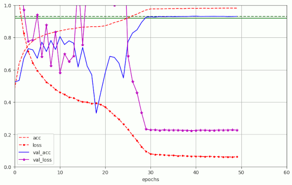
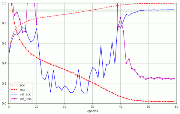
Plots for run10 in the above table are
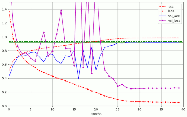
We see that the fluctuations in val_acc appear in a further condensed phase of 20 to 25 epochs. After a reduction of LR to LR ≤ 1.e-4 = α/10 the model converges and our threshold value of val_acc = 0.92 is passed at around epoch 30 – reproducibly and for a variety of parameter values. Admittedly in a rather narrow range …
Interpretation
Even though we pass our threshold of val_acc ≥ 0.92 in most of the above runs we do not reach higher values easily during the reduced number of epochs. In the runs above we started to reduce the LR already from epoch 0 onward. This leads on average to a shorter distance over which the model can move across the loss-hypersurface in comparison to longer runs. This may indicate that we reach a relatively flat valley on the loss hyper-surface in the direction of the loss gradient with a relatively low value of the gradient itself. But we do not reach the real loss minimum somewhere else in this valley due to the small number of remaining epochs and the very small LR. If you look at the eventual values of the loss for the training data reached e.g. in run 10, you find that it is by a factor of roughly 3 to 4 bigger than in the longer runs summarized by table 1.
Runs over 20 to 30 epochs
The following table summarizes the results of runs which I based on schedule with relatively long initial phases of high LR values before I applied the cosine shaped decline. For a typical example of the schedule’s forms see illustration 1 and the information given in the following table. As you I have reduced the number of epochs up to the end of the cosine decline even further. Runs 21 to 34 stretch only over 26 epochs.
Table 3 – runs over 20 to 35 epochs with a LR decline ahead of epoch 30
| # | epoch | acc_val | acc | epo best | val acc best | final loss | final val loss | shift | l2 | λ | α | LR reduction model |
| 14 | 27 | 0.92030 | 0.9567 | 32 | 0.92490 | 0.1010 | 0.2301 | 0.07 | 0.0 | 0.30 | 8.e-4 | [8.e-4, 0]lin[8.e-4, 16]cos[1.e-5, 28]lin[2.e-6, 34] |
| 15 | 27 | 0.92210 | 0.9614 | 30 | 0.92880 | 0.0892 | 0.2127 | 0.07 | 0.0 | 0.20 | 1.e-3 | [1.e-3, 0]lin[1.e-3, 16]cos[1.e-5, 28]lin[6.e-6, 34] |
| 16 | 24 | 0.92190 | 0.9611 | 30 | 0.92324 | 0.1021 | 0.2332 | 0.07 | 0.0 | 0.20 | 1.e-3 | [1.e-3, 0]lin[1.e-3, 14]cos[1.e-5, 24]lin[6.e-6, 34] |
| 17 | 23 | 0.92310 | 0.9590 | 29 | 0.92570 | 0.0903 | 0.2317 | 0.07 | 0.0 | 0.15 | 1.e-3 | [1.e-3, 0]lin[1.e-3, 14]cos[1.e-5, 24]lin[6.e-6, 34] |
| 18 | 23 | 0.92230 | 0.9539 | 26 | 0.92584 | 0.0928 | 0.2241 | 0.07 | 0.0 | 0.18 | 1.e-3 | [1.e-3, 0]lin[1.e-3, 14]cos[1.e-5, 24]lin[6.e-6, 32] |
| 19 | 23 | 0.92070 | 0.9558 | 31 | 0.92720 | 0.1018 | 0.2232 | 0.07 | 0.0 | 0.16 | 1.2e-3 | [8.e-4, 0]lin[1.2e-3, 8]lin[1.2e-3, 14]cos[1.e-5, 24]lin[6.e-6, 34] |
| 20 | 21 (!!) | 0.92170 | 0.9554 | 23 | 0.92340 | 0.1254 | 0.2303 | 0.07 | 0.0 | 0.18 | 1.25e-3 | [1.e-3, 0]lin[1.25e-3, 6]lin[1.25e-3, 10]cos[1.e-5, 20]lin[6.e-6, 30] |
| 21 | 21 (!!) | 0.92030 | 0.9529 | 23 | 0.92140 | 0.1340 | 0.2371 | 0.07 | 0.0 | 0.18 | 1.20e-3 | [1.e-3, 0]lin[1.20e-3, 5]lin[1.20e-3, 10]cos[1.e-5, 19]lin[6.e-6, 26] |
| 22 | 21 | 0.90090 | 0.9197 | 26 | 0.90110 | 0.2332 | 0.2976 | 0.07 | 0.0 | 0.50 | 1.20e-3 | [1.e-3, 0]lin[1.20e-3, 5]lin[1.20e-3, 10]cos[1.e-5, 19]lin[6.e-6, 26] |
| 23 | 20 | 0.91500 | 0.9546 | 24 | 0.91510 | 0.1252 | 0.2536 | 0.07 | 0.0 | 0.08 | 1.20e-3 | [1.e-3, 0]lin[1.20e-3, 5]lin[1.20e-3, 10]cos[1.e-5, 19]lin[6.e-6, 26] |
| 24 | 19 | 0.91470 | 0.9540 | 26 | 0.91470 | 0.1179 | 0.2651 | 0.07 | 0.0 | 0.10 | 1.e-3 | [1.e-3, 0]lin[1.e-3, 10]cos[1.e-5, 20]lin[6.e-6, 26] |
| 25 | 21 (!!) | 0.92060 | 0.9578 | 26 | 0.92080 | 0.1241 | 0.2358 | 0.07 | 0.0 | 0.15 | 1.0e-3 | [1.e-3, 0]lin[1.e-3, 12]cos[1.e-5, 20]lin[6.e-6, 26] |
| 26 | 26 | 0.86660 | 0.8754 | 26 | 0.86660 | 0.3690 | 0.3907 | 0.07 | 0.0 | 0.18 | 8.e-3 | [1.e-3, 0]lin[8.e-3, 5]lin[8.e-3, 10]cos[1.e-5, 20]lin[6.e-6, 26] |
| 27 | 23 | 0.89850 | 0.9229 | 26 | 0.89850 | 0.2268 | 0.2920 | 0.07 | 0.0 | 0.18 | 5.e-3 | [1.e-3, 0]lin[5.e-3, 5]cos[1.e-5, 20]lin[6.e-6, 26] |
| 28 | 21 | 0.90110 | 0.9211 | 24 | 0.90190 | 0.2262 | 0.2929 | 0.07 | 0.0 | 0.18 | 5.e-3 | [5.e-3, 0]cos[1.e-5, 20]lin[6.e-6, 26] |
| 29 | 20 | 0.91410 | 0.9520 | 26 | 0.91680 | 0.1356 | 0.2456 | 0.07 | 0.0 | 0.18 | 2.e-3 | [2.e-3, 0]lin[2.e-3, 4]cos[1.e-5, 20]lin[6.e-6, 26] |
| 30 | 20 | 0.91410 | 0.9534 | 26 | 0.91680 | 0.1356 | 0.2456 | 0.07 | 0.0 | 0.18 | 2.e-3 | [2.e-3, 0]lin[2.e-3, 12]cos[1.e-5, 20]lin[6.e-6, 26] |
| 31 | 22 | 0.91860 | 0.9414 | 25 | 0.91900 | 0.1687 | 0.2383 | 0.07 | 0.0 | 0.18 | 1.e-3 | [1.e-3, 0]lin[1.e-3, 12]cos[1.e-5, 20]lin[6.e-6, 26] |
| 32 | 21 | 0.90810 | 0.9351 | 25 | 0.90910 | 0.1837 | 0.2672 | 0.07 | 0.0 | 0.18 | 1.e-3 | [8.e-4, 0]lin[1.e-3, 5]lin[1.e-3, 10]cos[1.e-5, 19]lin[6.e-6, 26] |
| 33 | 19 (!!) | 0.92060 | 0.9434 | 25 | 0.92220 | 0.1252 | 0.2316 | 0.07 | 0.0 | 0.18 | 1.e-3 | [8.e-4, 0]lin[1.e-3, 5]lin[1.e-3, 12]cos[1.e-5, 20]lin[6.e-6, 26] |
| 34 | 23 | 0.92090 | 0.9554 | 26 | 0.92140 | 0.1355 | 0.2285 | 0.07 | 0.0 | 0.18 | 1.e-3 | [8.e-4, 0]lin[1.e-3, 5]lin[1.e-3, 14]cos[1.e-5, 20]lin[6.e-6, 26] |
In general, we no longer reach as high accuracy values for the training data as with longer runs. Consistently, the final loss values are significantly higher than in previous longer runs.
But, on the positive side, we pass our threshold for the validation accuracy val_acc ≥ 0.92 for some parameter settings already very early. Initial phases of a linearly rising LR followed by a subsequent plateau phase were introduced with run 19.
Plots for run 17 are
Runs 20 and 21 show that we can get the epoch where we pass our threshold down to Nepo = 21
Note, that the validation data were varied between run 20 and 21. Respective plots for run 20 are:
Plots for run 20 – 21 epochs to pass our threshold of val_acc ≥ 0.92
Plots for run 21 – 21 epochs to pass our threshold of val_acc ≥ 0.92
We note that small differences in parameters and a change of the validation data set may lead to differences in the fluctuation pattern ahead of the fast reduction of the learning rate. In run 20 we find only one extreme amplitude of the fluctuations between epochs 10 and 20.
Super-Convergence?
For some special parameter settings we can bring the number of required epochs for a validation accuracy of 0.92 down to Nepo = 21. This is sort of a success: We came very close to epoch numbers for which other publications claimed a so called “super-covergence” of their models – though for the SVG-optimizer. However, the above data show that with the present network setup we cannot reproduce this result convincingly, yet.
In the case of the scenarios investigated above I would therefore rather refrain from the term “super-convergence”. Runs 21, 25, 31, 32, 33, 34 show that slight changes in the schedule and changes in the validation set may hinder the ResNet model to pass our threshold value close to epoch 21 or before. It obviously is a rather delicate matter to reach a position on the loss hyper-surface close enough to the overall minimum within 21 epochs. On the other side it is no wonder that already small changes of the LR schedule become decisive, when we only have 21 epochs available to manage a plateau and a systematic decline of the learning rate.
So, did we see some kind of super-convergence? I would not say so …
Top accuracy values are not no longer reached
There is also a price we apparently have to pay for our “success”:
With our present approach we do not reach the optimum validation accuracy values any more. Remember that in longer runs (35 < Nepo < 60) we sometimes got values above val_acc=0.924 and sometimes even close to val_acc=0.93. Now, both the validation accuracy, the training accuracy and the loss for the training data only take sub-optimal values. In particular the high eventual loss values indicate that we do not come close enough to the minimum reached in longer runs.
What could we possibly improve to approach super-convergence and/or better validation accuracy values ?
The reader may have noticed that we control the decline of both the WD and the LR by one and the same schedule. The question is whether Keras implementation of optimizers allow us to separate a LR-schedule fro a WD-schedule. And what kind of effect that might have. Another point is that we have not managed momentum or used exponential moving momentum averages (ema) so far. A third idea might be to modify some elements of the ResNet itself.
Readers who have looked into details of the ResNet setup of R. Atienza may have seen that the “bottleneck” layer of the first Residual Unit [RU] of a new Residual Stack [RSN] just continues with the same number of maps which the preceding stack RSN-1 had on the output side. But we could go down by a factor 0.5 there and instead raise the number of maps on the output layer of the RUs of the new stack by a factor of 4 afterward. The bottleneck in the number of maps would then be more extreme between the following RUs (factor of 0.25). (See my post “ResNet basics – II – ResNet V2 architecture” for more information on the structure of a ResNetV2.) Such a change will be the topic of a forthcoming post in this series.
Another question that may come up is the kernel-size of the convolutional shortcut layer with stride=2 at the first RU of each RS. A further point concerns the transition between the core ResNet and the fully connected network part following it. There standard recipes proclaim some crude pooling towards a fixed number of neurons in a flattened layer. This could be disputed.
Raising the WD-parameter significantly does not help
Runs 22 and 23 shows that raising the WD parameter λ to high values or choosing a rather low value does not help.
This shows that we do need a significant side drift created by WD and added to the weight value correction during gradient descent. The WD related “drift” vector points to the origin of origin of the coordinate system of the multidimensional weight space. It changes both the direction and value of the correction vector in comparison to a purely gradient controlled one. This may change the path towards a minimum e.g. at saddle points of the loss hyper-surface. But the added correction vector of WD obviously must have a length in a rather narrow range defined by λ-values
This range may be specific for the CIFAR10 dataset.
Raising the LR-parameter significantly does not help
One could be tempted to think that raising the initial learning rates to a very high plateau value like 0.008 or 1.e-2 may help. But this is not true. Runs 26 to 30 prove this.
Actually, LR values in the range
are optimal values for reducing the loss quickly and most efficiently per iteration step in the beginning of the runs. So, it is not astonishing that much bigger values as e.g. used in 1Cycle approaches do not help us much in our case.
Conclusion: Clever LR schedules allow for very short trainings, but we miss optimal accuracy values
A comparison of the results achieved in this post for our testcase of a ResNet56v2, a mini-batch size of BS=64 and the CIFAR10 dataset with the results of preceding posts shows:
- Instead of a piecewise linear LR schedule we can equally well use a schedule which includes a cosine shaped decline phase.
- Pure Weight Decay (without any L2 regularization) in the Keras version of the AdamW optimizer helps us to achieve reasonable validation accuracy values val_acc = 0.92 within a relatively short training. If we need to fight for one or two percent improvement we need runs with a number of epochs between 35 and 50.
- We should apply optimal values of the learning rate through relatively long initial phases. In our case the values were given by a relatively small range 8.e-4 ≤ LR ≤ 1.1e-3.
- Weight decay in the sense of AdamW appears to be important. Also here the relevant parameter had to be chosen in a relatively narrow range of 0.15 ≤ λ ≤ 0.25 to achieve optimal results.
- For some parameter settings we can bring the number of training epochs Nepo required to pass a threshold of val_acc = 0.92 for Cifar10 down to even Nepo = 21. But such a reduction depends too sensitively on details of the LR schedule and on other parameters, yet, and can therefore not be called super-convergence.
- Both the learning rate as well as the weight decay must be diminished by one to two orders of magnitude ahead of a final (short) phase of the training. So far we have coupled a reduction of the weight decay to the LR schedule.
- All data indicate that diminishing the LR over two magnitudes ahead of a final convergence phase may relatively abruptly stop the progress of the model towards a (global) minimum reached in longer runs. The relatively high eventual loss values indicate that we got stuck in an area of the loss-hypersurface with a relatively small gradient.
We have come a long way in comparison to results provided by R. Atienza in a text book on Deep Learning: Reducing training from around 120 epochs down below 25 epochs by a clever LR schedule means something in term of calculation time and energy consumption. But there is still room for improvement.
In forthcoming posts we should therefore try to implement some changes in the network itself. This includes changes of the convolutional shortcut layers and changes for the transition of the core ResNet to the fully connected layers at the network’s end. Such changes are easy to implement; they will be the topic of the next post.
AdamW for a ResNet56v2 – VI – Super-Convergence after improving the ResNetV2
The title already suggests that super-convergence is achievable at last. So stay tuned …
Afterward we should also investigate the effect of a more extreme bottleneck. In addition we should analyze the impact of changed batch sizes, a separation of the schedules for the declines of WD and LR. In addition we should have a look at a competitive optimizer – namely SVG.
I also want to point out that the relatively narrow ranges of the parameters for an initial LR and WD stand in some contrast to other publications on Weight Decay (see the literature lists in the preceding posts). Whether this is in part due to the Keras implementation of WD for AdamW remains unclear. The fact that the reduction of the LR over 2 orders of magnitude more or less stops the models approach to a minimum sets a question mark behind some implementations of 1Cycle approaches. To achieve optimal values of a validation or test accuracy may simply require more than 20 epochs of training. But have a look at the next post in this series …
Addendum: The fluctuations in the validation loss are a real effect
In the precedent post I have already investigated whether the observed huge fluctuations were caused by some deficits of the set of evaluation samples. This was not the case. In the experiments descrived above the validation sets were individual, but stratified ones per run. In the meantime I got a mail from a reader asking whether the fluctuations could be the result of some kind of error in the data delivered by Keras at the end of each epoch, e.g. by delivering data of the final batch or subtleties of the averaging. After having saved models after each epoch and having compared the val_loss data evaluated by Keras vs. evaluation loss values calculated by myself, I can assure that Keras3 works how it should. At the end of an epoch an averaged value over all (mini-) batches is presented. So, there are no effects in the sense that Keras would show some kind of non-averaged values.
Another point is that the LR schedule is applied after each iteration step, i.e. after each batch processed during gradient descent. This has the effect that some batches experience larger corrections than the late ones in an epoch. However, any possible statistical trend induced thereby is reduced due to sample shuffling between the epochs.