This series is about a ResNetv56v2 tested on the CIFAR10 dataset. In the last post
AdamW for a ResNet56v2 – I – a detailed look at results based on the Adam optimizer
we investigated a piecewise constant reduction schedule for the Learning Rate [LR] over 200 epochs. We found that we could reproduce results of R. Atienza, who had claimed validation accuracy values of
- 0.92 < val_acc < 0.93
with the Adam optimizer. We saw a dependency on the batch size [BS] – and concluded that BS=64 was a good compromise regarding achievable accuracy and runtime.
But we needed typically more than 85 epochs to get safely over an accuracy level of val_acc=0.92. Our objective is to reduce the number of epochs as much as possible to reach this accuracy level. In the present post we try to bring the required number of epochs down to 50 epochs by four different measures:
- Target 50 epochs: Reduction of the number of training epochs by shorter phases of a piecewise constant LR schedule / application of the Adam optimizer
- Target 50 epochs: Application of a piecewise linear LR schedule and of the Adam optimizer without weight decay
- Target 50 epochs: Application of a piecewise linear LR schedule and of the Adam optimizer with weight decay
- Target 50 epochs: Application of the AdamW optimizer – but keeping L2 regularization active
Three additional approaches
- Target 50 epochs: AdamW optimizer – without L2-regularization, but with larger values for the weight decay
- Target 50 epochs: Cosine Annealing schedule and changing the Batch Size [BS] in addition
- Target 30 epochs: Application of a 1Cycle LR schedule
will be the topics of forthcoming posts.
All test runs in this post were done with BS=64 and image augmentation (with shift=0.07), as described in the first post of this series. I did not use the ReduceLROnPlateau() callback which R. Atienza applied in his experiments. The value for the accuracy reached on the validation set of 10,000 CIFAR10 samples is abbreviated by val_acc.
Layer structure of the ResNet56v2
For the experiments discussed below my personal ResNet generation program was parameterized such that it created the same layer structure for a ResNet56v2 as the original code of Atienza (see [1] and the first post of this series). I have checked the layer structure and number of parameters thoroughly against what the code of Atienza produced.
 Total params: 1,673,738 (6.38 MB)
 Trainable params: 1,663,338 (6.35 MB)
 Non-trainable params: 10,400 (40.62 KB)
I have consistently used this type of ResNet56v2 model throughout the test runs described below (with BS=64).
Trial 1: Shortening the first phase of a piecewise constant LR schedule for optimizer Adam
A simple approach to achieve a shorter training is to reduce the number of epochs during which we keep the learning rate value LR = 1.e-3 constant. In a first trial we reduce this phase to 60 epochs. The data of previous runs (see post I) let us hope that we nevertheless will get a fast convergence to a good accuracy value between epochs 60 and 70. And indeed:
782/782 ━━━━━━━━━━━━━━━━━━━━ 0s 27ms/step - acc: 0.9634 - loss: 0.3070
Epoch 64: val_acc improved from 0.91970 to 0.92230, saving model to /.../cifar10_ResNet56v2_model.064.keras
782/782 ━━━━━━━━━━━━━━━━━━━━ 24s 30ms/step - acc: 0.9634 - loss: 0.3070 - val_acc: 0.9223 - val_loss: 0.4433 - learning_rate: 1.0000e-04

The solid green line defines the value 0.92, the dotted green line 0.93. The model obviously passed an accuracy value of val_acc=0.922 at epoch 64 and reached a maximum value val_acc=0.9254 at epoch 83. So, we have shortened the number of required epochs to reach the accuracy level of 0.92 already by around 20 epochs. Without doing much :-).
However, when we move on to a piecewise constant schedule like this one: {(epoch, LR)} = {(40, 1.e-3), (60, 1.e-4)} we fail and reach
- epoch 48: val_acc=0.914, epoch 64: val_acc=0.9166,
only. It appears that this time we have reduced the learning rate LR too early.
Adam with weight decay?
Adam offers an option to enable a regularizing method called “weight decay“. In this post we do not consider details of this method. We just take it as a further option for regularization. The interested user will get much more information about L2-regularization and pure “weight decay” in the next post.
The question, which concerns us here, is whether we can improve the convergence by using Adam with weight decay. And actually, already a small weight decay factor of
- wd = 5.e-4 and an ema_momentum = 0.8
helped. Below I specify the used piecewise constant scheme by tuples (epoch, LR). The first element gives a target epoch, the second a learning rate value.
- LR-schedule: (40, LR=1.e-3), (50, LR=1.e-4), (60, LR=1.e-5)
- val_acc: epoch 51: val_acc=0.92160 => epoch 54: val_acc=0.92270.
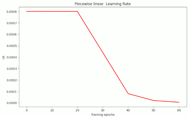
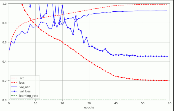
A small adjustment of the LR schedule gave us the following result:
- LR-schedule: (38, LR=1.e-3), (48, LR=1.e-4), (55, LR=1.e-5), (60, LR=5.e-6)
- val_acc: epoch 49: val_acc=0.92260 => epoch 53: val_acc=0.92450
For the latter run the plots below show the LR schedule and the evolution of the accuracy, of the (training) loss, the validation accuracy and of the validation loss:

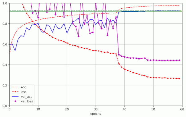
This success was achieved by very simple means. It proves that it is worthwhile to care about Adam in combination with weight decay in further experiments. But regarding the piecewise constant LR schedule the message is that we should not reduce the number of epochs in the first two phases much more.
Note the strong variation of val_loss during the first phase in the above experiments. We have discussed this point already in the last post. We will return to the topic of strong oscillatory fluctuations in the next posts of this series.
Trial 2: Runs with with Adam, L2 regularization, piecewise linear LR schedule, no weight decay
With the next experiments I wanted to reach a level of val_acc=0.92 with a piecewise linear schedule like the following one:
- LR-schedule: {(20, LR=8.e-4), (40, LR=8.e-5), (50, LR=2.e-5), (60, LR=5.e-6)}
I applied the pure Adam optimizer (as implemented in Keras) with default values and no weight decay.
To make a longer story short: I needed a relatively strong L2 contribution. Otherwise I did not reach my objective within 50 epochs, but only came close to the threshold of 0.92 (val_acc=0.916 to 0.918). But not above it …
| # | epoch | acc_val | acc | epo best | val acc best | shift | l2 | wd | ema mom | reduction model |
| 1 | 51 | 0.91620 | 0.9956 | 53 | 0.91170 | 0.07 | 1.e-4 | – | – | [8.e-4, 20][4.e-4, 30][1.e-4, 40][1.e-5, 50][4.e-6, 60] |
| 2 ?? | 51 | 0.91940 | 0.9854 | 57 | 0.92090 | 0.07 | 1.5e-4 | – | – | [8.e-4, 20][8.e-5, 40][1.e-5, 50][5.e-6, 60] |
| 3 | 50 | 0.92040 | 0.9842 | 60 | 0.92070 | 0.07 | 1.8e-4 | – | – | [8.e-4, 20][8.e-5, 40][1.e-5, 50][5.e-6, 60] |
| 4 | 51 | 0.9200 | 0.9850 | 55 | 0.92190 | 0.07 | 1.85e-4 | – | – | [8.e-4, 20][8.e-5, 40][1.e-5, 50][5.e-6, 60] |
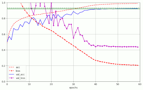
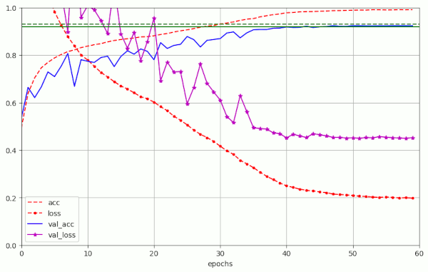
| 5 | 48 | 0.92020 | 0.9818 | 60 | 0.92300 | 0.07 | 2.e-4 | – | – | [8.e-4, 20][8.e-5, 40][1.e-5, 50][5.e-6, 60] |
| 6 | 48 | 0.92050 | 0.9839 | 57 | 0.92420 | 0.07 | 2.e-4 | – | – | [8.e-4, 20][8.e-5, 40][1.e-5, 50][5.e-6, 60] |
| 7 | 44 | 0.92090 | 0.9755 | 59 | 0.92420 | 0.07 | 2.e-4 | – | – | [8.e-4, 20][8.e-5, 40][1.e-5, 50][5.e-6, 60] |
| 8 | 53 | 0.92000 | 0.9836 | 58 | 0.92050 | 0.07 | 3.e-4 | – | – | [8.e-4, 20][8.e-5, 40][1.e-5, 50][5.e-6, 60] |
| 9 | 51 | 0.91460 | 0.9766 | – | 0.91460 | 0.07 | 4.e-4 | – | – | [8.e-4, 20][8.e-5, 40][1.e-5, 50][5.e-6, 60] |
| 10 | 50 | 0.91780 | 0.9758 | 58 | 0.91950 | 0.07 | 4.5e-4 | – | – | [8.e-4, 20][8.e-5, 40][1.e-5, 50][5.e-6, 60] |
| 11 | 52 | 0.91240 | 0.9721 | 57 | 0.91380 | 0.07 | 6.e-4 | – | – | [8.e-4, 20][8.e-5, 40][1.e-5, 50][5.e-6, 60] |
The evolution of run nr. 5 is shown in the following graphics:
Note: In the runs nr. 3 for l2=1.8 and run nr. 8 for l2=3e-4, respectively, the value of val_acc=0.92 was just touched at epoch 50, but did not stay above 0.92 between epochs [51,59[. During the experiments nr. 9 to nr. 11 we did not even reach the aspired accuracy level. So, it seems that the variation of the L2-parameter “l2” should be kept in the range
- 1.9e-4 <= l2 < 3.e-4
to reach our goal. This is a rather narrow range.
Interpretation: I. Loshilov and F. Hutter [8] have shown (for another type of network) that convergence to good accuracy values with the Adam optimizer (without weight decay) is possible, only, when the initial learning rate and the L2 parameter are kept in a relatively narrow diagonal band in the plane of (initial LR-values, L2-values). The band indicates a correlation between L2 and LR values (see [8] for details). We observe signs of this correlation here, too.
Side remark: For further comparisons with [8] please note that we work with a standard (un-branched) ResNet network (of depth 56) in this post series. This model has 1.7 million parameters, only. The authors of [8], instead, employed a branched ResNet (of depth 26) with 11.6 million parameters (according to sect. 6 in [8]).
Another aspect is that a strong contribution of a L2 regularization term to the loss typically leads to both a flattening and broadening of the loss environment close to the minimum. In addition they the minimum value itself rises in comparison to an undisturbed loss. In comparison to a situation with a pronounced and sharply defined undisturbed minimum, both effects are counterproductive regarding the achievable accuracy.
We will come back to the eventual loss level reached with and without L2 regularization and a chance to improve accuracy by avoiding L2-modification of the loss during the next posts. Both theoretically and numerically.
Trial 3: Adam with weight decay, L2 regularization, piecewise linear LR schedule
Again, it was interesting to see whether adding weight decay would come with some improvement. Meaning: Would we achieve our goal even with a low value of l2 = 1.e-4 and an additional small amount of weight decay ?
This was indeed the case:
| # | epoch | acc_val | acc | epo best | val acc best | shift | l2 | wd | ema mom | reduction model |
| 1 | 49 | 0.92040 | 0.9835 | 54 | 0.92460 | 0.07 | 2.e-4 | 4.e-3 | 0.99 | [8.e-4, 20][8.e-5, 40][2.e-5, 50][5.e-6, 60] |
| 2 | 51 | 0.92020 | 0.9896 | 54 | 0.92080 | 0.07 | 1.e-4 | 1.e-5 | 0.99 | [8.e-4, 20][8.e-5, 40][2.e-5, 50][5.e-6, 60] |
| 3 | 42 | 0.92000 | 0.9801 | 51 | 0.92480 | 0.07 | 1.e-4 | 5.e-4 | 0.98 | [8.e-4, 20][8.e-5, 40][2.e-5, 50][5.e-6, 60] |
| 4 | 50 | 0.92010 | 0.9888 | 53 | 0.92130 | 0.07 | 1.e-4 | 1.e-3 | 0.98 | [8.e-4, 20][8.e-5, 40][1.e-5, 50][1.e-5, 60] |
| 5 | 49 | 0.92130 | 0.9876 | 58 | 0.92310 | 0.07 | 1.e-4 | 1.e-4 | 0.98 | [8.e-4, 20][8.e-5, 40][2.e-5, 50][6.e-6, 60] |
Run 3 had a remarkable sequence of
- (0.92, 42), (0.9226, 43), (0.9232, 47), (0.9244, 50), (0.9246, 51), (0.9250, 60).
Such sequences appeared with other settings, too. Below you see a table with data I got from a sequence of other earlier test runs.
| # | epoch | acc_val | acc | epo best | val acc best | shift | l2 | wd | ema mom | reduction model |
| 1 | 50 | 0.92350 | 0.9848 | 58 | 0.92600 | 0.08 | 1.e-4 | 1.e-5 | 0.98 | [8.e-4, 30][1.5e-5, 40] |
| 2 | 48 | 0.92070 | 0.9803 | 57 | 0.92180 | 0.08 | 1.e-4 | 1.e-5 | 0.98 | [8.e-4, 30][1.e-4, 40][1.e-5, 50][1.e-6, 60] |
| 3 | 50 | 0.9210 | 0.9870 | 56 | 0.92180 | 0.08 | 1.e-4 | 1.e-5 | 0.98 | [8.e-4, 20][4.e-4, 30][4.e-5, 40][4.e-6, 50][1.e-6, 60] |
| 4 | 50 | 0.92170 | 0.9843 | 52 | 0.92190 | 0.08 | 1.e-4 | 1.e-5 | 0.98 | [8.e-4, 20][4.e-4, 30][8.e-5, 40][1.e-5, 50][4.e-6, 60] |
| 5 | 49 | 0.92400 | 0.9870 | 55 | 0.92481 | 0.07 | 1.e-4 | 1.e-5 | 0.98 | [8.e-4, 20][4.e-4, 30][8.e-5, 40][1.e-5, 50][5.e-6, 60] |
| 6 | 50 | 0.92180 | 0.9878 | 53 | 0.92350 | 0.07 | 1.e-4 | 1.e-5 | 0.99 | [8.e-4, 20][4.e-4, 30][8.e-5, 40][1.e-5, 50][5.e-6, 60] |
| 7 | 49 | 0.92110 | 0.9883 | 56 | 0.92180 | 0.07 | 1.e-4 | 1.e-5 | 0.95 | [8.e-4, 20][4.e-4, 30][8.e-5, 40][1.e-5, 50][5.e-6, 60] |
| 8 | 49 | 0.92270 | 0.9888 | 59 | 0.92360 | 0.07 | 1.e-5 | 1.e-5 | 0.98 | [8.e-4, 20][4.e-4, 30][8.e-5, 40][1.e-5, 50][5.e-6, 60] |
| 9 | 49 | 0.92230 | 0.9870 | 60 | 0.92230 | 0.07 | 1.e-4 | 1.e-5 | 0.98 | [8.e-4, 24][4.e-4, 32][8.e-5, 40][1.e-5, 50][5.e-6, 60] |
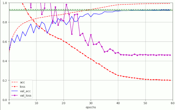
| 10 | 49 | 0.92390 | 0.9876 | 56 | 0.92410 | 0.07 | 1.e-4 | 7.e-4 | 0.98 | [8.e-4, 20][4.e-4, 30][8.e-5, 40][1.e-5, 50][5.e-6, 60] |
| 11 | 49 | 0.92390 | 0.9876 | 56 | 0.92410 | 0.07 | 1.e-4 | 1.e-4 | 0.98 | [8.e-4, 20][4.e-4, 30][8.e-5, 40][1.e-5, 50][5.e-6, 60] |
The plot for run nr. 10 in the latter table looked like:
I forgot to integrate the green border lines at that time. Sorry, …
Trial 4: Runs with AdamW, L2 regularization and piecewise linear LR schedule
Let us switch to the optimizer AdamW. According to I. Loshilov and F. Hutter [8] and the author of [4] the effects of weight decay are consistently implemented in this optimizer. I will have a closer look at the math behind all this in a forthcoming post. For now we just apply AdamW in its Keras implementation.
As long as we employ the L2 mechanism and activate weight decay, our network deals with two types of regularization in parallel. Therefore, I keep the weight decay parameter “wd” relatively small during the next experiments:
- 1.e-4 <= wd <= 4.e-3.
Note that 4.e-3 is the default value in Keras.
What do we expect? Well, I would say, a slight improvement in comparison to Adam. The following table gives you some results of six different test runs.
| # | epoch | acc_val | acc | epo best | val acc best | shift | l2 | wd | ema mom | reduction model |
| 1 | 50 | 0.91980 | 0.9825 | 55 | 0.92100 | 0.07 | 1.e-4 | 1.e-4 | 0.99 | [8.e-4, 20][4.e-4, 30][8.e-5, 40][4.e-5, 50][5.e-6, 60] |
| 2 | 50 | 0.9205 | 0.9838 | 58 | 0.92300 | 0.07 | 2.e-4 | 4.e-3 | 0.99 | [8.e-4, 20][8.e-5, 40][4.e-5, 50][4.e-6, 60] |
| 3 | 50 | 0.9201 | 0.9900 | 59 | 0.92100 | 0.07 | 1.e-4 | 4.e-3 | 0.99 | [8.e-4, 20][8.e-5, 40][1.e-5, 50][5.e-6, 60] |
| 4 | 49 | 0.92220 | 0.9823 | 53 | 0.92370 | 0.07 | 2.e-4 | 4.e-3 | 0.99 | [8.e-4, 20][8.e-5, 40][2.e-5, 50][5.e-6, 60] |
| 5 | 44 | 0.922160 | 0.9830 | 51 | 0.92360 | 0.07 | 1.e-4 | 5.e-4 | 0.98 | [8.e-4, 20][8.e-5, 40][2.e-5, 50][7.e-6, 60] |
| 6 | 46 | 0.92270 | 0.9846 | 57 | 0.92510 | 0.07 | 1.e-4 | 1.e-4 | 0.99 | [8.e-4, 20][8.e-5, 40][2.e-5, 50][5.e-6, 60] |
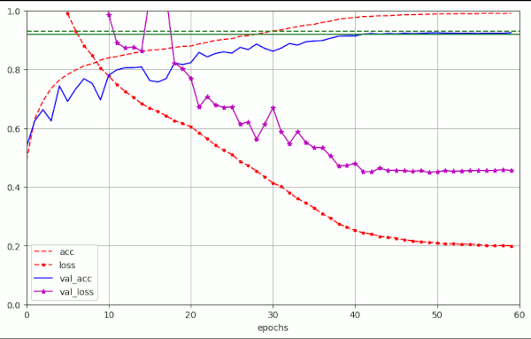
Obviously, it was possible to reproducibly reach acc_val=0.92 latest at epoch 50. But in some cases we achieved our goal significantly earlier. The plot below depicts the evolution of run nr. 5 for AdamW as an example:
Note that the 5th run for AdamW corresponds closely to run nr. 5 in the previous table for Adam based runs.
Some experiments showed that it is better to raise the ema_momentum to 0.99 with wd <= 1.e-4. See the plot for run nr. 6 in the table.
So, there is some variation with the the parameters named. However, there are multiple parameter combinations which bring us into our momentary target range of 50 epochs for val_acc=0.92.
The main message so far is that we do not see any really noteworthy improvement of runs with AdamW in comparison to runs using Adam with a properly set weight decay parameter (in its Keras implementation). This might be due to the still dominant impact of the L2 regularization. We will try a different approach in the next posts.
Summary
Observation 1: A reduction of epochs by a faster shrinking learning rate in a piecewise constant schedule is possible
We can reduce the number of epochs for a ResNet56v2 (built according to Atienza [1]) to reach a value of val_acc=0.92 to around epoch 50 just by moving the transition from LR=1.e-3 to LR=1.e-4 in a piecewise schedule to epoch 40. However, we needed Adam with weight decay to achieve our goal.
Observation 2: A piecewise linear LR reduction schedule is working well
A piecewise linear LR reduction after epoch 20 works even better – both with the Adam and the AdamW optimizer. We can get the number of epochs consistently down to 50 for reaching val_acc=0.92.
Observation 3: Adam seems to couple the initial learning rate to L2-values
If you do not use weight decay with the Adam optimizer you may have to raise the level of L2 regularization. However, regarding validation accuracy, the range of optimal L2-values for a given initial learning LR is limited.
Observation 4: Weight decay is important – also for the Adam optimizer
We need weight decay to press the number of epochs down below 50 to reach at least a level of val_acc >= 0.92 safely and reproducibly for a variety of hyper-parameter settings.
Observation 5: Adam and AdamW with weight decay and L2-regularization work equally well
As long as L2-regularization is active Adam with weight decay works equally well as AdamW with similar wd parameter values. But note: The weight decay parameter was kept relatively small in all our experiments (i.e. below 4.e-3) so far.
Observation 6: Do not make the LR too small too fast
All runs which converged to good accuracy values had LR values of LR > 8.e-5 up to epoch 40 and LR > 1.e-5 up to epoch 50.
Addendum, 12.06.2024: Observation 5 raises the interesting question whether Adam with weight decay and AdamW are implemented the same way in Keras. I have not yet analyzed the code, but there are some indications on the Internet that AdamW and Adam indeed are they same in Keras with the exception of the default value for weight decay. See e.g. these links:
Is AdamW identical to Adam in Keras?
AdamW and Adam with weight decay
Conclusion
By some simple tricks as
- a piecewise linear LR schedule, weight decay and an adjustment of L2-regularization strength
we can bring the required number of epochs Nepo to reach a validation accuracy level of val_acc >= 0.92 down to or below
Nepo ≤ 50.
This is already a substantial improvement in comparison to what R. Atienza achieved in his book. We should, however, not be too content. Some ideas published in [2] to [8] are worth to check out. A first point is that the authors of [8] have suggested to use AdamW without any L2-regularization. A second point is that they also favored a cosine based LR reduction scheme. In the next posts of this series I will explore both options. Afterward we will also study the option of super-convergence.
But a topic we first have to cover in more detail is the difference between L2-regularization and pure “weight decay”. This is the topic of the next post.
Links and literature
[1] Rowel Atienza, 2020, “Advanced Deep Learning with Tensorflow 2 and Keras”, 2nd edition, Packt Publishing Ltd., Birmingham, UK
[2] A.Rosebrock, 2019, “Cyclical Learning Rates with Keras and Deep Learning“, pyimagesearch.com
[3] L. Smith, 2018, “A disciplined approach to neural network hyper-parameters: Part 1 — learning rate, batch size, momentum, and weight decay“, arXiv
[4] F.M. Graetz, 2018, “Why AdamW matters“, towards.science.com
[5] L. N.. Smith, N. Topin, 2018, “Super-Convergence: Very Fast Training of Neural Networks Using Large Learning Rates“, arXiv
[6] S. Gugger, J. Howard, 2018, fast.ai – “AdamW and Super-convergence is now the fastest way to train neural nets“, fast.ai
[7] L. Smith, Q.V. Le, 2018, “A Bayesian Perspective on Generalization and Stochastic Gradient Descent”
[8] I. Loshchilov, F. Hutter, 2018, “Fixing Weight Decay Regularization in Adam“, arXiv