Orthogonal projections of multidimensional ellipsoids – VI – considerations and vector generation for numerical experiments in four dimensions

After our recent excursion to Schur complements, some readers may wish to get a visual confirmation of our rather theoretical results. As usual in this blog, we will perform some numerical experiments. To get started, I will restrict my efforts to the projection of an ellipsoid from a 4-dimensional Euclidean space down to three- and two-dimensional sub-spaces. In a later post, I will abandon the restriction of 4-dimensions.
The main objective of the forthcoming numerical experiments is to show that we can really produce the hulls of the ellipsoid’s projection image either by using Schur complements or by calculating the positions of tangential points on the multidimensional ellipsoid and projecting them down onto the target space. In this post, we only prepare such experiments. I briefly consider required calculation steps and explain some aspects of the generation of points on the ellipsoid. In the next post I will show the calculated hulls of the projection images of a specific ellipsoid embedded in the ℝ⁴.

On the fly, I will also cover the switching of coordinate axes, which was used in post IV of this series. For our numerical experiments, we have to handle this step by respective transformations. The procedures I am going to describe support the analysis of multidimensional statistical distributions that approach a multivariate normal distribution within a limited inner core. I will return to the theory of such MVN-cores in the near future.

A general hint to avoid misunderstandings:
A 3-dimensional ellipsoid encapsulates a 4-dimensional volume by a closed 3-dimensional “surface“. Also the unit sphere 𝕊³ of the ℝ⁴ represents a 3-dim surface manifold. Both figures can not be plotted directly and should not be confused in the following sections with their lower dimensional counterparts the reader may be used to.

Previous posts

Restriction and suppositions

Why a preliminary restriction to four dimensions? The reason is two-fold:
(1) We need to numerically generate representative vectors of ellipsoids in a n-dimensional space. Lazy people like me want to limit respective efforts.
(2) The minimum number of dimensions to reasonably test a projection from a n-dimensional space to a (n-2)-dimensional sub-space is n=4.

Working in the ℝ⁴

We will work in the Euclidean ℝ⁴. We choose 4 base (unit) vectors e_i (1 ≤ i ≤ 4) in the order { e₁,e₂,e₃,e₄} and set up an original Cartesian Coordinate System “OCS” to cover the ℝ⁴. Switching the order of coordinate axes, e.g. to { e₁,e₄,e₃,e₂ }, will lead us to a changed coordinate system, which I call “SCS” below. SCS and OCS are related by a very simple kind of transformation, which can easily be performed by matrix multiplications in numerical experiments. In more complex cases you may have to change the positions of more than two vectors.

Bring base vectors spanning the projection’s target space into leading positions

The reason why we may want to switch the order of the base vectors is that we want to get those unit vectors which cover the target sub-space of our projection to be the first ones in the order of the coordinate system. As we have sen in post IV, this simplifies the math operations to get the proper Schur complement of the ellipsoid’s quadratic form matrix. In the example mentioned before we are interested in a projection down to the (1,4) plane spanned by the vectors {e₁,e₄} – and change to a SCS build upon the base {e₁,e₄,e₃,e₂}.
Hint: While reordering the base vectors try to keep the original order of the base vectors spanning your target sub-space to avoid a change of the ellipsoid’s orientation in plots.

Projections and sub-spaces

To cover the case of a projection to a 3-dim sub-space, we will simply use a sub-space S_P3 orthogonal to a select base vector e_k, i.e. S_P3 ⊥ e_k. To investigate a projection to a 2-dim sub-space, we instead select a target space S_P2 spanned by two selected base vectors {e_m, e_n} picked from our set of base vectors.

Using projections down to target spaces spanned by base vectors is no major restriction to generality. For a well defined target space of the projection orthogonal to some vectors, we could always have calculated and chosen unit vectors to span this sub-space. In addition: For a general matrix of the ellipsoid’s quadratic form the ellipsoid’s main axes will be rotated against the 4 base vectors. As long as we do not choose the axes to be the major axes of the ellipsoid the situation therefore is already a pretty general one. So, it is enough to change the order of the axes in some calculations. Remember that we need to do this anyway to calculate the required Schur complement acc. to the recipe given in post IV.

Programming

I did the programming with Python. Plots were made with the help of Matplotlib. I distributed a varying number of points on the surface in a simple and non-homogeneous manner (see the respective section below). This will lead to clearly visible asymmetry effects in the volume covered by the ellipsoidal surfaces. However, will not hamper our main objectives. The readers are trusted to be able to create respective Python code by themselves. Regarding the Schur complements as a method to predict the ellipsoidal hull of an ellipsoid’s projection image, I will give numerical numbers and compare the inverse Schur complement to a specific block of the original inverse quadratic form matrix (or of covariance matrices, if you like to think in terms of multivariate distributions).

Blocks of the quadratic form matrix for an ellipsoid in the ℝ⁴

The matrix defining the quadratic form Q (= Σ^-1) of the ellipsoid in our OCS with un-changed order of the base vectors {e₁,e₂,e₃,e₄} is assumed to have a block structure like

\[ \pmb{\operatorname{Q}} \,\, \left( \, \equiv \pmb{\operatorname{\Sigma}}^{-1} \, \right) \,=\, \begin{pmatrix} \pmb{\operatorname{Q}}_{yy} & \pmb{\operatorname{Q}}_{yz} \\ (\pmb{\operatorname{Q}}_{yz})^T & \pmb{\operatorname{Q}}_{zz} \end{pmatrix} \,. \tag{1} \]

Q defines the ellipsoid as a collection of 4-dim vectors to points on the manifold:

\[ \begin{align} & \text{vectors } \pmb{x}_e \text{ of 3-dim ellipsoid } E\,\text{ in the } \mathbb{R}^4 : \\[10pt] & \pmb{x}_{e} \in E = \left\{ (\pmb{x}_e)^T \,\, | \,\, \pmb{x}_e \, \pmb{\operatorname{Q}} \, \pmb{x}_{e} \,=\, 1 \, \right\} \subset \mathbb{R}^4 \,. \tag{2} \end{align} \]

In case of a projection onto a 2-dim sub-space, all blocks are (2×2) matrices, with Q_yy ad Q_zz being symmetric, invertible and pos.-definite. Note also: In case of a projection onto a 3-dim sub-space, Q_yy is a (3×3) matrix, Q_yz a (3×1) matrix and Q_zz a (1×1) scalar.

The original ellipsoid can be constructed by applying a linear transformation A to vectors of the unit sphere 𝕊³, with A fulfilling

\[ \pmb{\operatorname{Q}}^{-1} \,\, \left( \,=\, \pmb{\operatorname{\Sigma}} \,\right) \,=\, \pmb{\operatorname{A}} \pmb{\operatorname{A}}^{T} \,. \tag{3} \]

Numpy provides functions for the required Cholesky decomposition. Note that an original Q will become subject of a transformation to a coordinate system SCS with a switched order of the coordinate axes. However, we would fill the same 3-dim “surface” of the ellipsoid independent of whether we generate data points with Q or its transformed matrix Q_S; see below.

Generative matrix A

A is a generative matrix for points on the original ellipsoid. We create vectors of the ℝ⁴‘s unit sphere 𝕊³ and apply the generative matrix A to these vectors to get points on the ellipsoid. Transformations of Q to account for a switching of the order of coordinate vectors will in some cases only affect the orientation of the resulting volume of the projection figure, but not its general shape. We will, however, see below that a non-homogeneous filling of the original ellipsoidal manifold may imprint certain patterns into the ellipsoid and its projection images.

Transformation to a coordinate system with switched order of base vectors

Let me briefly show how to transform from an OCS to a specific SCS. We will use such a transformation for Schur complement calculations of the four possible projections to 3-dim sub-spaces and all 6 projections to 2-dim coordinate planes. As an example, let us again assume that we want to perform a projection to the (1,4)-coordinate plane spanned by {e₁,e₄}. To determine the required Schur complement correctly, we need to switch the order of base vectors such that e₁ and e₄, which span the target space, become the first two vectors of our base vector tuple. therefore, we reorder the unit vectors to the sequence {e₁,e₄,e₃,e₂}. This means we describe the ellipsoid in a new coordinate system in which axes 2 and 4 have been switched in comparison to our original OCS.

Transformation matrix: The required transformations matrix S is actually a rather simple one. S just contains the original base unit vectors in the new order as lines (or columns). E.g. S for switching e₄ (= (0,0,0,1)^T with e₂ = (0,1,0,0)^T, matrix S looks like

\[ \pmb{\operatorname{S}} \,=\, \begin{pmatrix} 1 & 0 & 0 & 0 \\ 0 & 0 & 0 & 1 \\ 0 & 0 & 1 & 0 \\ 0 & 1 & 0 & 0 \end{pmatrix} \,. \tag{4} \]

You find the explanation in books on Linear Algebra. In a more general case you may need to reorder more of the vectors. The resulting matrices are all symmetric and orthonormal. But as said above: Try to keep the original order of the base vectors spanning the target space.

Transformation of the ellipsoid’s vectors to the SCS-system: We transform vectors given in the OCS to our SCS by applying S:

\[ \pmb{x}_{Se} \,=\, \pmb{\operatorname{S}} \, \pmb{x}_e \, . \tag{5} \]

This transformation just switches coordinates. Try it out.
Note: The vector elements in the projection’s target sub-space are after this transformation given by the first three or two components of x_Se, when you perform a projection down to a 3-dim or 2-dim sub-space, respectively.

Transformation of the quadratic form matrix Q to the SCS-system: We get the transformed quadratic form matrix (Q_S) in the system SCS as

\[ \pmb{\operatorname{Q}}_{\pmb{\operatorname{S}}} \,=\, \pmb{\operatorname{S}} \, \pmb{\operatorname{Q}} \, \pmb{\operatorname{S}}^T \,. \tag{6} \]

This transformation switches the positions of the matrix elements as required. The generative matrix A_S in system SCS is given by a Cholesky decomposition of [Q_S]^-1 :

\[ \pmb{\operatorname{Q}_S}^{-1} \,=\, \pmb{\operatorname{A_S}} \, [\pmb{\operatorname{A_S}}]^{T} \,. \tag{7} \]

Determining the Schur complement of Q for the selected target coordinate plane correctly: In the SCS system we can safely apply the recipes of post IV to calculate the Schur complement. Let us again regard a projection to a coordinate plane given by the first two unit vectors in the SCS. In our example the (1,4)-coordinate plane given by vectors {e₁,e₄}. The quadratic form Q_Ps of the projection’s hull in the coordinate plane is then given by the Schur complement [Q_S/Q_S,_zz] of Q_S:

\[ \pmb{\operatorname{Q_{Ps}}} \,=\, \left[ \pmb{\operatorname{Q}}_{\pmb{\operatorname{S}}} / \pmb{\operatorname{Q}}_{\pmb{\operatorname{S}},zz} \right] \,. \tag{8} \]

We get the generative matrix A_Ps in the lower dimensional target space by a Cholesky decomposition of [Q_Ps]^-1 :

\[ [\pmb{\operatorname{Q_{Ps}}}]^{-1} \,=\, \pmb{\operatorname{A}}_{Ps} \, \pmb{\operatorname{A}}_{Ps}^T \,. \tag{9} \]

Note: Acc. to post V, the inverse matrix [Q_Ps]^-1 (in the CCS with the reordered axes) should be equivalent to the upper left block of [Q_S]^-1, i.e. [[Q_S]^-1]_yy.

\[ [\pmb{\operatorname{Q_{Ps}}}]^{-1} \,=\, [\pmb{\operatorname{Q}}_S^{-1}]_{yy} \,. \tag{10} \]

This is worth checking separately in our forthcoming experiments.

Identifying tangential points on the surface

Let us assume that we have already performed the transformation to the SCS. Previous posts in this series showed that tangential points on the ellipsoid, which give us the hull of the projection’s resulting volume in the target space, can be derived from vectors s^t describing the intersection of a specially oriented sub-space with the unit sphere 𝕊³. In case of a projection to a 3-dim subspace S_P3 ⊥ e_k, we must look at the intersection of yet another 3-dim S_k sub-space orthogonal to the vector A_S^-1 e_k with the unit sphere 𝕊³

\[ \begin{align} & \text{tangential points of projection onto 3-dim sub-space : } \\[10pt] & \quad S_k \perp \pmb{\operatorname{A_S}}^{-1} \pmb{e}_k \quad\Rightarrow \,\, \pmb{s}^t \in \left( S_k \, \cap \, \mathbb{S}^3 \right) \,. \tag{11} \end{align} \]

The intersection is given by a 𝕊² in S_k.

In the case of a projection onto a coordinate plane S_P2 spanned by { e_m,e_n } we must instead consider the the intersection of a subspace S_m,n with the 𝕊³

\[ \begin{align} & \text{tangential points of projection onto 2-dim sub-space : } \\[10pt] & S_{m,n} \perp \pmb{\operatorname{A_S}}^{-1} \, \pmb{e}_m \,\,\land \,\, S_{m,n} \perp \pmb{\operatorname{A_S}}^{-1} \, \pmb{e}_n \quad\Rightarrow \,\, \pmb{s}^t \in \left( S_{m,n} \, \cap \, \mathbb{S}^3 \right) \,. \tag{12} \end{align} \]

In the latter case the intersection is given by a unit circle 𝕊¹ in S_m,n. Vector’s of the intersections, i.e. of the named unit spheres, can be used to create the tangent point vectors u_e^t with the help of the already available generative matrix A_S :

\[ \pmb{u}^t_e \,=\, \pmb{\operatorname{A_S}} \, \pmb{s}^t \,. \tag{13} \]

These points can then be projected to the target space to give us the hull of the ellipsoid’s projection image.

**Determination of orthogonal unit base vectors for the special sub-spaces S_k or S_m,n**

A remaining numerical task is the determination of orthogonal unit vectors spanning S_k or S_m,n, respectively. This task is not so trivial as one may expect, because these vectors must of course be orthogonal to the vector A_S^-1 e_k or to the tuple {A_S^-1e_m, A_S^-1e_n }, respectively. The easiest way to get such vectors is to perform a SVD-decomposition (see here) of a matrix G whose rows are formed by e_k or e_m,e_n :

\[ \pmb{\operatorname{G}} \,=\, \pmb{\operatorname{U}} \,\pmb{\operatorname{D}}\,\pmb{\operatorname{V}}^T \,. \tag{14} \]

In the case of a projection to a 3-dim sub-space G is a (1×4)-matrix, in case of a projection onto a 2-dim coordinate plane G is a (2×4)-matrix. In both cases V^T results in a (4×4) orthogonal matrix. The last 3 or 2 rows of V^T represent orthonormal (4-dim) vectors spanning S_k or S_m,n, respectively. The reason why V^T has this property is explained in good books on Linear Algebra. For our experiments we just take this property as given. If you want you can check the orthogonality properties in your own codes.

Three methods to create the hull of the projected figure in the sub-space

According to the considerations in the previous posts of this series, we have 3 methods available to construct the hull of the ellipsoid’s projection image in the target sub-space (after a proper reordering of the coordinate axes and respective unit vectors) :

We determine [[Q_S]^-1]_yy, apply a Cholesky decomposition to get a valid A_Ps and apply this matrix to vectors of the unit sphere (𝕊² or 𝕊¹) in the lower dimensional target space(s) of our projection(s).
Determine the Schur complement [Q_S/Q_S,_zz] and invert it. Take the result [Q_S/Q_S,_zz]^-1, apply a Cholesky decomposition to get a valid A_Ps and apply this matrix to vectors of the unit sphere (𝕊² or 𝕊¹) of the lower dimensional target space(s) of our projection(s).
Apply a Cholesky decomposition to [Q_S]^-1 to get a valid A_S. Then determine proper 4-dim base vectors of the special sub-spaces S_k and S_m,n, use these special base vectors to create unit spheres in these sub-spaces. Afterward apply A_S to these vectors and project the resulting points down to our target sub-space.

In our planned numerical experiments we should test all 3 methods to show the consistency of our mathematical results gathered in posts IV and V.

Filling an ellipsoidal surface in n > 3 dimensions with data points

One of the problems for the setup of a reasonable numerical experiment regarding a (n-1)-dim ellipsoidal surface in the ℝⁿ is posed by the following question:

How do we fill the ellipsoidal surface densely and regularly with data points? The points should in the ideal case have equal distances from each other.

To my knowledge this problem has no simple solution in the general case n > 3.

Because we know that one can generate an ellipsoid from a unit sphere we might be content with a solution for a (n-1)-sphere. But even the task of filling a unit sphere 𝕊^n-1 in multiple dimensions (n > 3) with roughly equidistant points is not a trivial one. While the problem has been solved for the ℝ³ and the 𝕊² (see e.g. [1]), a general solution in more dimensions requires bigger efforts. See e.g. the ingenious idea of Daniel P. in [2]. I was just too lazy to program his suggestion of distributing points along a multidimensional spiral. However, some readers may be more eager to follow Daniel’s recipe.

Now, you may say: Why not use a simple parameterization in radius and (n-1) angles of spherical coordinates for the 𝕊³ of the ℝ⁴? Well, this is exactly what I am going to do in my laziness. The way to proceed is described at Wikipdia; see [3]. It is relatively easy to program this kind of parameterization of the 𝕊³.

However, the effects of the resulting non-homogeneous point distribution already on the 𝕊³ get clearly visible during projections. Sometimes resulting in interesting patterns:
The point concentrations will e.g. be maximal at the original poles of the chosen spherical coordinate system, where one axis is chosen to provide a kind of global latitude angle. Spheres at constant latitude will have a greater point density density. Original lines/areas at other constant parametric angles will also become prominent in the projections.

The following plot shows a projection of the parameterized 𝕊³-manifold onto the four 3-dim sub-spaces spanned by base-vectors of the ℝ⁴. Per sub-space we see three different perspectives :

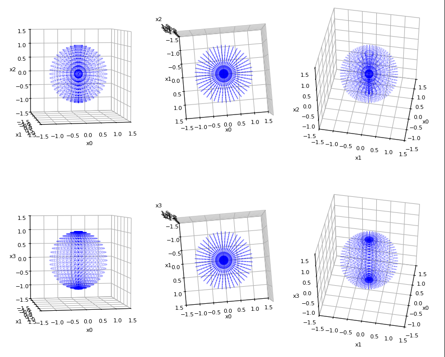
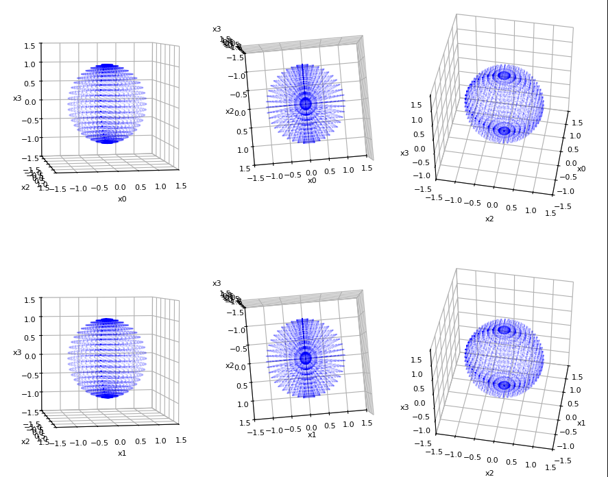
And here the projections to the six 2-dim coordinate planes:

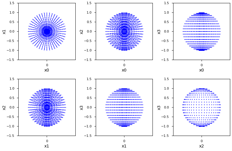
In the plots above, I have used around 21300 points to cover the 𝕊³.

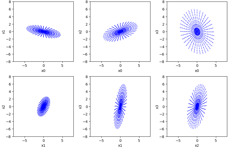
This generation comes with a degree of freedom. We can switch the orientation of the axis and angles for point generation, too:

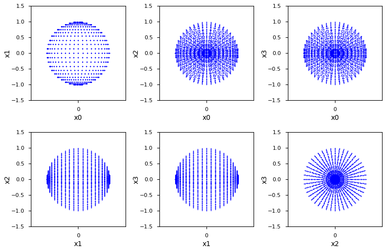
The construction of the ellipsoids from these points of the 𝕊³ with the help of a generating matrix A will rotate and stretch the figure in 4 dimensions. But we will nevertheless detect clear traces of the non-homogeneously filling of the 𝕊³-manifold. Just to give you a first impression:

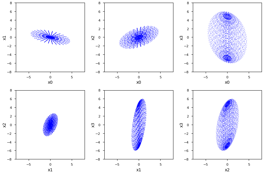
In the plots above, I have used 15 pts per angle range instead of 22. It should become clear that we can imprint certain pattern onto the ellipsoid and its projections by choosing a certain way of point generation before and/or after the transformation to a SCS. When we create the ellipsoid after the switch to a SCS, we can e.g. decide to get all projections a look like in the above left corner.

Funny, isn’t it ? All these pictures indicate already an elliptic surface or hull of the projection figures. In th enext post we will calculate them.

Continuous and transparent elliptical hull in 3D-plots?

We add one more tool to our toolbox for the intended numerical experiments. The discussed angle parameterization of the unit sphere 𝕊² to construct the hull via method 1 or 2 for a projection to a 3-dim (!) target space has an advantage: It allows for building a common 2-dim Matplotlib meshgrid as a base for the (x,y,z) coordinates of the hull’s points. Based upon such a coordinate representation over a meshgrid, we can use Matplotlib’s function “plot_surface()” to create a continuous and transparent surface manifold.

Summary

The mathematical description of the orthogonal projection of multidimensional ellipsoids is associated with Schur complements. Numerical experiments to prove the mathematical concepts require a series of steps as transformations, matrix calculations and other tools. We have described the basic procedures in this post for the projections of a 3-dim ellipsoidal manifold embedded in the ℝ⁴ to lower dimensional sub-spaces.

A basic step is the generation of points on the 𝕊³ unit sphere of the ℝ⁴. From these points we can calculate vectors to points on the ellipsoid. Following a parameterization of the 𝕊³ via equidistant angles of spherical coordinates leads to asymmetric patterns imprinted onto the projections of respective points of the ellipsoid. However, we expect that all outmost points of the projected figures will be connected by an ellipsoidal hull, e.g. calculated from Schur complements. In the next post of this series, I will show that this really is the case. Stay tuned …