Orthogonal projections of multidimensional ellipsoids – VII – experimental checks of projections from a 4-dimensional space to sub-spaces

This post series covers the topic of orthogonal projections of ellipsoids from their embedding multidimensional space down to sub-spaces. In this post we will verify some of our mathematical results by a numerical experiment: We will compute the projections of an ellipsoid from its embedding 4-dimensional (Euclidean) space down to 3- and 2-dimensional sub-spaces. We will check with the help of graphical tools that the hull of a projection image is yet another lower dimensional ellipsoid. We will also verify that the quadratic form of the projected ellipsoidal hull is indeed given by a Schur complement of the quadratic form matrix of the original ellipsoid. In addition we are going to show that the inverse of the Schur complement is given by a sub-matrix of the inverse of the ellipsoid’s original quadratic form matrix.

Requirements: Aside of the math, the reader should be familiar with some steps required to perform the numerical experiments. I have discussed some important elements already in post VI of this series. The notation in this post will follow the one of post VI.

Previous posts

Suppositions and numerical approaches

We will work in the Euclidean ℝ⁴. We choose standard base vectors e_i (1 ≤ i ≤ n) of a Cartesian coordinate system “OCS”, in which we place our ellipsoid. In the OCS the ellipsoid is defined by a quadratic form matrix Q. We restrict our study of projections to sub-spaces S_P3 and S_P2 spanned by selected base vectors:
A target S_P3 of a projection down to a 3-dim sub-space will be chosen to be orthogonal to a selected base vector, e.g. S_P3 ⊥ e_k. To investigate a projection down to a 2-dim sub-space, we choose a S_P2 spanned by two selected base vectors e_n and e_m. Due to the freedom to rotate the original ellipsoid and adjust its quadratic form matrix this selection of target spaces does not restrict generality.

We have, however, already seen that it is rather useful to change the order of the base vectors such that the vectors spanning the projection’s target space get a leading position in an ordered tuple of the 4 base vectors. This corresponds to switching the order of the coordinate axes of our original OCS system, in which the quadratic form matrix Q for our ellipsoid was given. I.e., for a particular projection we eventually work in a new coordinate system “SCS” with a different order of coordinate axes in comparison to OCS. All vectors and matrices originally defined in OCS have to be transformed to this SCS. See post VI for details. Note that a SCS is specific for a certain projection and its target space.

A general warning: A three dimensional ellipsoid is a figure that has a 3-dimensional “surface”. The unit sphere 𝕊³ of the ℝ⁴ has 3-dim surface. Both figures can not be plotted directly and should not be confused with their lower dimensional counterparts.

The original quadratic form matrix of the ellipsoid in the ℝ⁴

In the Cartesian coordinate system OCS we have a matrix

\[ \pmb{\operatorname{Q}} \,=\, \begin{pmatrix} \pmb{\operatorname{Q}}_{yy} & \pmb{\operatorname{Q}}_{yz} \\ (\pmb{\operatorname{Q}}_{yz})^T & \pmb{\operatorname{Q}}_{zz} \end{pmatrix} \,, \tag{1} \]

which defines our ellipsoid E in the ℝ⁴:

\[ \begin{align} & \text{vectors } \pmb{x}_e \text{ of 3-dim ellipsoid } E\,\text{ in the } \mathbb{R}^4 : \\[10pt] & \pmb{x}_{e} \in E = \left\{ (\pmb{x}_e)^T \,\, | \,\, \pmb{x}_e \, \pmb{\operatorname{Q}} \, \pmb{x}_{e} \,=\, 1 \, \right\} \subset \mathbb{R}^4 \,. \tag{2} \end{align} \]

We use the following concrete matrix, which the reader may recognize from other previous experiments (see e.g. post I):

\[ \pmb{\operatorname{Q}} \, = \, \begin{pmatrix} \,\,21 & \,-4 & \,\,\, \, 6 & \, -5 \\ \,-4 & \,\,\,\, 3 &\,\,\, \, 2 & \,\,\, \, 5 \\ \,\,\,\,6 & \,\,\,\, 2 & \,\,\,\, 7 & \,\,\, \, 6 \\ \,-5 & \,\,\,\, 5 &\,\,\, \, 6 & \,\,\, \, 36 \end{pmatrix} \tag{3} \,. \]

A Cholesky decomposition of Q^-1 gives us a generative matrix A which allows us to create vectors x_e from vectors s₃ of the unit sphere 𝕊³ via

\[ \pmb{x}_e \,=\, \pmb{\operatorname{A}} \, \pmb{s}_3, \quad \text{with} \,\,\, \pmb{\operatorname{Q}}^{-1} \,=\, \pmb{\operatorname{A}}\, \pmb{\operatorname{A}}^T, \,\, \pmb{s}_3 \in \mathbb{S}^3 \,. \tag{4} \]

In post VI, I have discussed the possible appearance of characteristic patterns in the projection images. Such patterns result from filling the 𝕊³ with discrete points at discrete angles of spherical coordinates. I.e. the ellipsoid will be covered by discrete points reflecting lines of constant angle(s) on the 𝕊³.

Switching to the SCS coordinate system: For a particular projection, we switch from the OCS-system to a system SCS with properly changed order of axes and base vectors, such that the unit vectors which span the target space of the projection come first and determine the first two or three components of all vectors. Thereby we reproduce the assumptions of our mathematical considerations in posts IV and V. To cover the transition between the OCS and our SCS properly, we must apply a proper transformation matrix S to all vectors and matrices as described in post VI.

Steps to get plots of the ellipsoid’s projection images and their hulls

I briefly list up major steps for numerical experiments, which I encoded in Python functions:

Step 0: In the original coordinate system OCS, get the generative matrix A via a Cholesky decomposition of Q^-1. Generate vectors s₃ of the unit sphere 𝕊³ via equidistant angles of spherical coordinates in 4 dimensions. Create a bunch of vectors x_e of the ellipsoid from vectors s₃ of the unit sphere 𝕊³ with the help of A acc. to eq. (4). The projections of these data down onto the target sub-spaces will exhibit different patterns, resulting from the asymmetric filling of the 𝕊³.
Loop over the different target spaces (either four 3-dim or six 2-dim sub-spaces (i.e. coordinate planes in our approach).
- Step 1: Select the unit base vectors spanning the target sub-space of the current projection. Switch the order of the coordinate axes accordingly and perform a transformation of the matrix Q to the new coordinate system SCS via a matrix S (Q -> Q_S=SQS^T). Also transform the ellipsoid’s vectors (x_Se = Sx_e) and the unit vectors (e_Si = Se_i). Note again: The SCS and matrix S are specific for the projection and its target space.
- Step 2: Calculate the elements of [Q_S]^-1 and perform a Cholesky decomposition to get a generation matrix A_S in the SCS.
- Step 3.1 (optional): In the SCS generate new vectors w₃ of the unit sphere 𝕊³ via equidistant angles of spherical coordinates in 4 dimensions. Chose a specific unit vector to define the latitude related angle to select a specific filling pattern for the ellipsoidal manifold. The filling of the 𝕊³ can thus be made specific for the current SCS and the projection. E.g., the same type of filling pattern can be chosen for each projection. See post VI.
  Apply A_S to the vectors w₃ of 𝕊³ to get vectors x_Se of the ellipsoid’s 3-dim manifold in the ℝ⁴. These vectors will carry a distinct pattern, which will also appear in the projection images.
- Step 4A – alternative to 4B, 4C – hull computation using tangential points:
  In the SCS, compute vectors v_k= [A_S]^-1(Se_k), with k marking those base vectors not spanning the projection’s target space in the OCS (!); see post IV for the math. Use a SVD according to the recipe in post VI to calculate orthonormal vectors of special sub-spaces S_k in the SCS orthogonal to the v_k. The Se_k are the last 3 or 2 base unit vectors of the SCS base. Intersect the special sub-spaces S_k with the 𝕊³ in the SCS. Create a sufficient number of vectors s^t in the intersection. Apply A_S to these vectors to derive vectors of tangential points u_S^t on the ellipsoid. The projections of these tangential points define the ellipsoidal hull in the projection’s target space. But see also a later section below.
- Step 4B – alternative to 4A, 4C – hull computation by inverse Q-matrix: Read the sub-matrix [Q_S^-1]_yy off matrix Q_S^-1, use a Cholesky decomposition to get a creative matrix A_P in the projection’s target sub-space and create the hull’s ellipsoid in the target space from vectors s_p of the sub-space’s unit sphere.
- Step 4C – alternative to 4A, 4B – hull computation by Schur complement: Compute the Schur complement [Q_S/Q_S,_zz] of Q_S to get the quadratic form matrix Q_P of the projection’s hull in the target sub-space. Invert Q_P, afterward apply a Cholesky decomposition to get a generating matrix A_P and create the hull’s ellipsoid in the target space from vectors s_p of the latter’s unit sphere (𝕊² or 𝕊¹, depending on the dimensionality of the target space).
- Step 5: Project either the original ellipsoid points given by x_{_Se} or the pattern imprinted x_Se down to the target space. Plot these data and the projections of the tangential points (given by the u_S^t ) for the hull in the target space.
- Step 6 – optional for projections onto 3-dim sub-spaces: In case of a 3-dim target space you may use a meshgrid of angles for getting s_p vectors and resulting ellipsoidal data. This will allow you to create a continuous surface with Matplotlib’s function plot_surface; see post VI.

Comparison of the Schur complement with a sub-matrix block of the inverse Q_S^-1 of the quadratic form matrix

An important relation we have derived in this post series is given in eq. (30) of post V and eq. (10) of post VI:

\[ [\pmb{\operatorname{Q_{P}}}]^{-1} \,=\, [\pmb{\operatorname{Q}}_S^{-1}]_{yy} \,. \tag{5} \]

For all projections we have to compute the difference matrix D. I just give you the elements of D for two examples:

Difference matrix D for projection to 2-dim sub-space (coordinate plane):

5.55111512e-17 9.71445147e-17
4.16333634e-17 0.00000000e+00

Difference matrix D for projection to 3-dim sub-space (coordinate plane):

1.11022302e-16 6.93889390e-17 6.93889390e-17
6.93889390e-18 0.00000000e+00 3.81639165e-17
1.11022302e-16 0.00000000e+00 2.77555756e-17

As it makes no sense to show differences in the 16th or 17th digit after the decimal point (in 32 Bit accuracy), the reader just has to trust me that the numerical data showed that this relation was perfectly fulfilled for all projections.

Due to the equivalence, results for the hull computed with method 4B or 4C will be totally equal.

Computation of tangential points

Triggered by the question of a reader, I briefly repeat what to do in the case of a projection to a coordinate plane: In the SCS-system with the reordered base-vectors, you have to pick the last ones not spanning the projection’s target space. Let us call the unit vectors e_s3 ad e_s4. Note that in the SCS a unit vector e_si has the same form as e_i in the OCS.

Apply [A_S]^-1 to these vectors, i.e. create e_w1=[A_S]^-1e_s1 and e_w2=[A_S]^-1e_s. Build a matrix W (here a 2×2)-matrix) out of these vectors, with each of the vectors marking one row; you can use Numpy’s function vstack() to achieve this. Apply a SVD decomposition for this matrix W=UDV^T; the last two rows of V^T give you two orthonormal base vectors. These vectors span a 2-dim subspace S_w, whose vectors are orthogonal to both e_w1 and e_w2. The intersection of this space (a plane) with the 𝕊³ of the SCS is given by a unit-circle 𝕊¹ of S_w. Create vectors for this circle and apply A_S to these vectors to get vectors u_S^t of the tangential points on the ellipsoid in the SCS.

Results for projections onto 2-dim coordinate planes

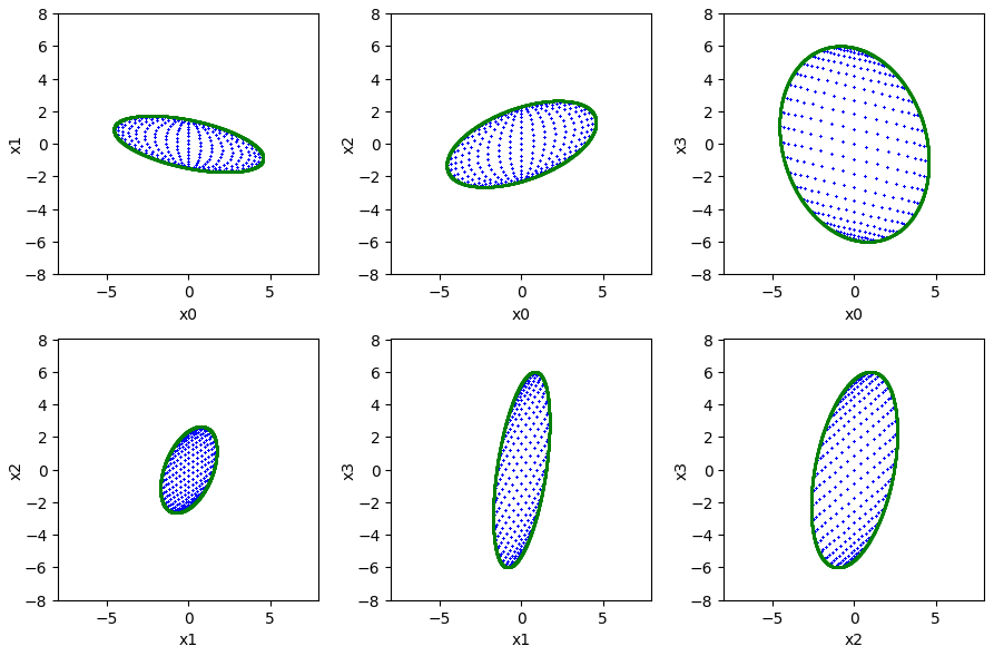
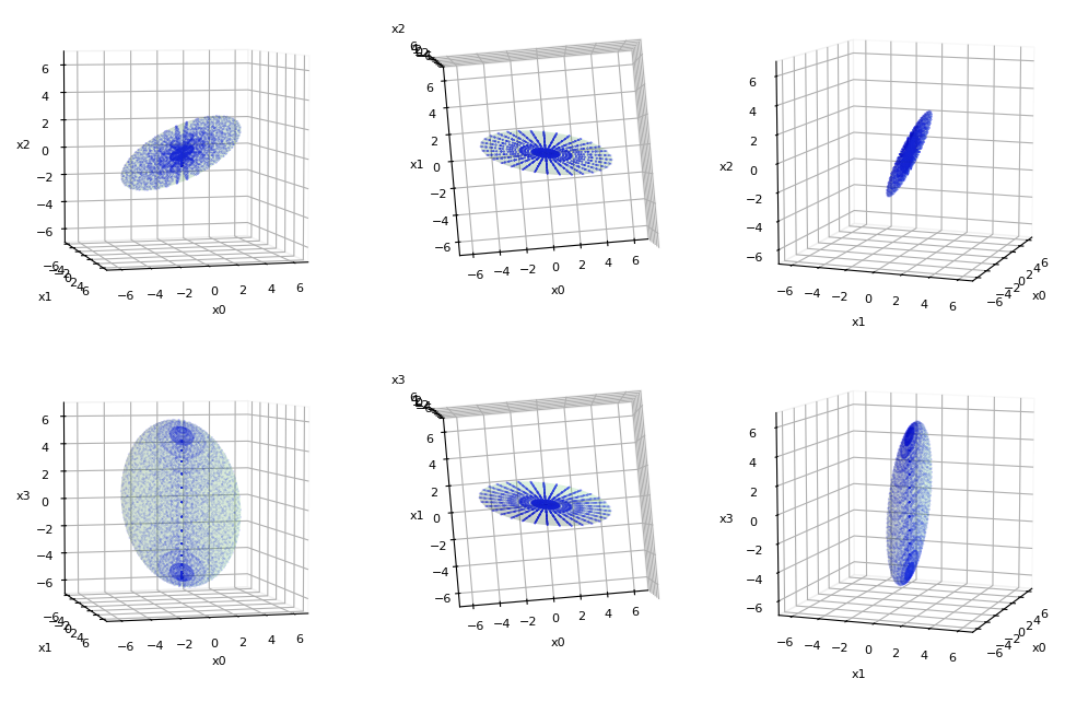
The following plots show you the results of projections on the six coordinate planes of the ℝ⁴. I first show you plots for which I have used projections of the x_{_Se}-data of the ellipsoid. For the filling of the 𝕊³, I have used only 16 distinct and equidistant values for each of the four angles in the range [0, π] to clearly mark resulting patterns for the different projections. Note: It is exactly one overall filling pattern of the 𝕊³ that affects all of the projections of the once fixed x_{_Se}-data.

The plots show us different projections of the points on the original ellipsoid from the ℝ⁴ down to the six coordinate planes. The red line corresponds to 1000 data points calculated with method 4A, i.e. via determining tangential points on the ellipsoid and projecting them. Note that the hull resulting from the computed tangential points perfectly fits the elliptic border line which the out-most blue points of the ellipsoid indicate:

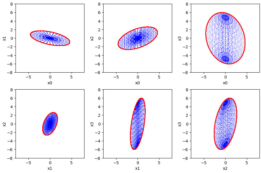
Note that in the plots “x0” marks the coordinate axis given by e₁ in the original OCS (!) and so on.

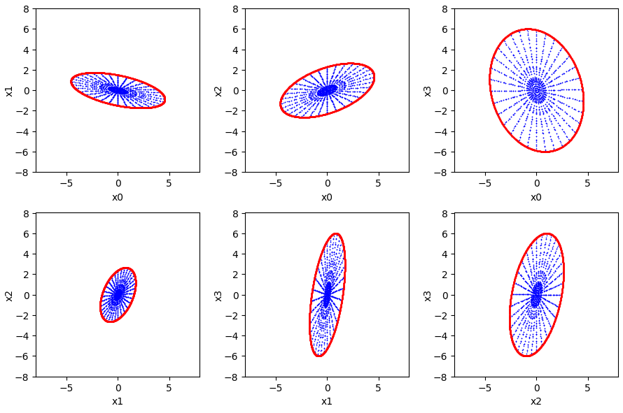
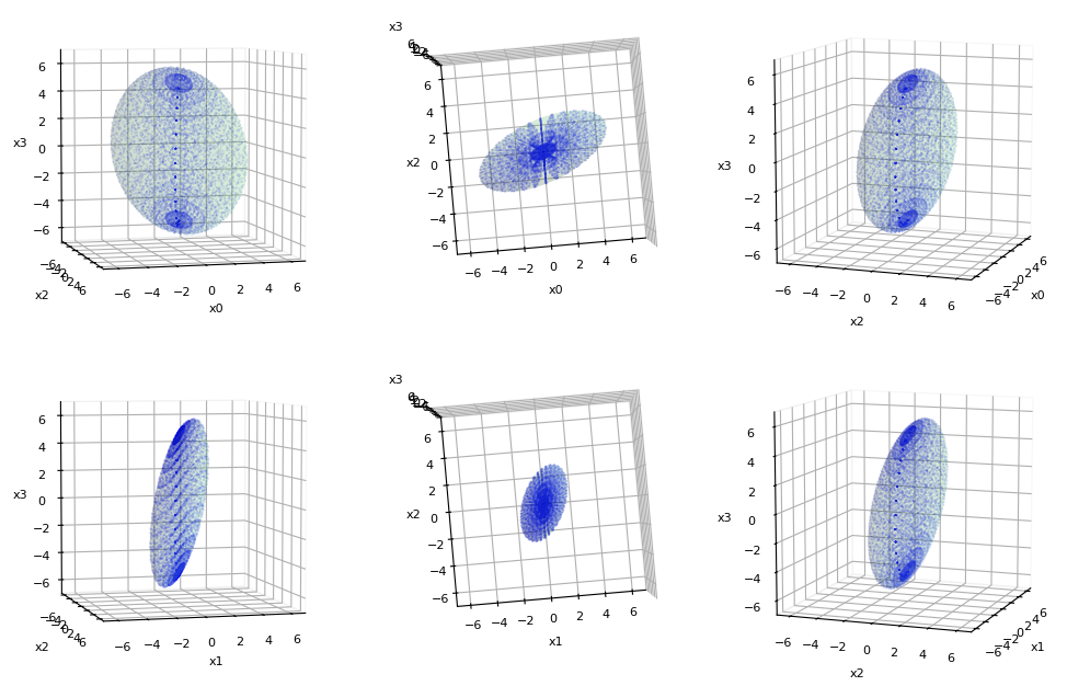
By using x_Se data, we can also enforce a common pattern for each of the projections. This time the filling of the 𝕊³ and the creation of points on the ellipsoid is done in a separate and equal way for each of the different SCS. The hull was again computed via method 4A:

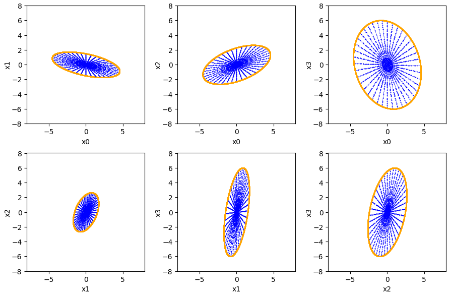
For 20 pts per angle and for a different filling pattern of the of the 𝕊³ we get (hull computed again by method 4A):

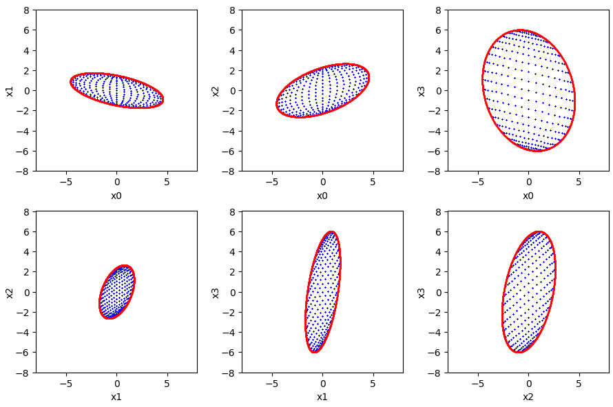
The next plot shows a calculation of the hull via the Schur complement and its inverse by method 4C:

The next plots show the hull which results when we read off sub-matrix [Q_S^-1]_yy directly and use method 4B :

As expected all of the methods 4A, 4B, 4C give us the same elliptic hull of the ellipsoid’s projection images in the different coordinate planes. This proves the consistency of the mathematical considerations and the applicability of the formulas derived in this post series.

Visualization of the tangential points in a 3D plot

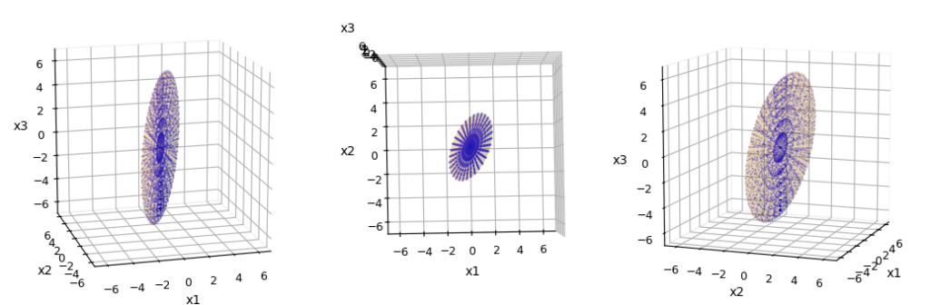
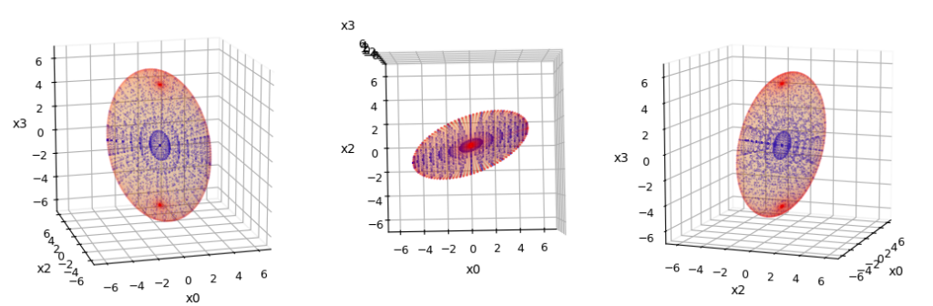
We cannot directly visualize the tangential points on the ellipsoid in the ℝ⁴. However, we can use an intermediate projection to three dimensional sub-spaces to get some impressions of how they circumvent the ellipsoid.

Let us for example take the eventual projection of the ellipsoid to the (x1,x3)-plane of the OCS and compute the tangential points determining the hull of the projection image in this coordinate plane.

Note that due to the remaining two axes, there are two 3D-projections associated with this plane. On the resulting ellipsoids in 3 dimensions we see the projections of the tangential points plotted in red.

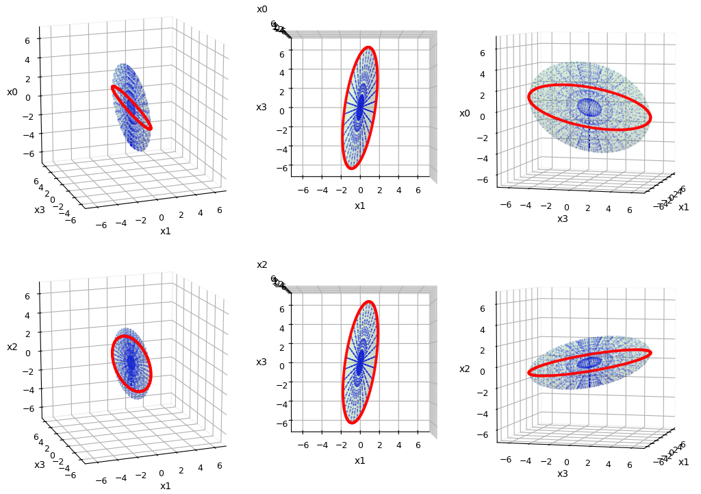
I have added a transparent ellipsoidal surface in light green to the blue data of the ellipsoid. The 3-dimensional transparent hull was computed using method 4B and an angle-based meshgrid. It was plotted by Matplotlib’s function plot_surface.

Because the tangential points were computed for the (x1, x3)-plane, we expect that the hull computed from these points perfectly fits the out-most projected points of the ellipsoid for an orthogonal view onto this coordinate plane. The middle plots in the perspectives presented above show that this indeed is the case.

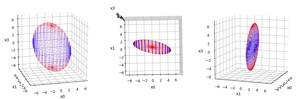
For a different filling pattern of the of the 𝕊³ and less tangential points (transparent hull again by method 4B):

Now, you may ask: What about tangential points for a projection on a 3-dim sub-space?

Projection onto 3-dim sub-spaces

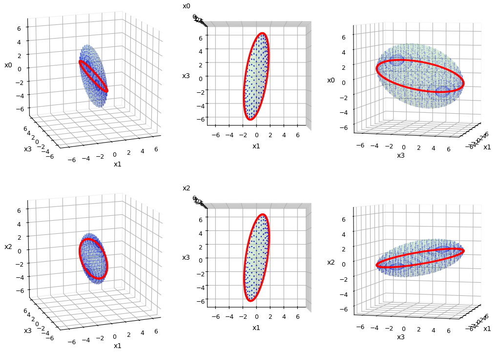
The construction of a continuous transparent hull in a 3-dim target space can in the easiest way be done by again using method 4B to construct its data by filling a 𝕊² in the SCS on a meshgrid. Actually, the transparent 3-dim hull was created by method 4B from 200 pts of the 𝕊² in the S_k-subspace of the SCS. Due to symmetry reasons this is in our approach equivalent to directly filling a 𝕊² in the target space (I leave it to the reader to prove this) :

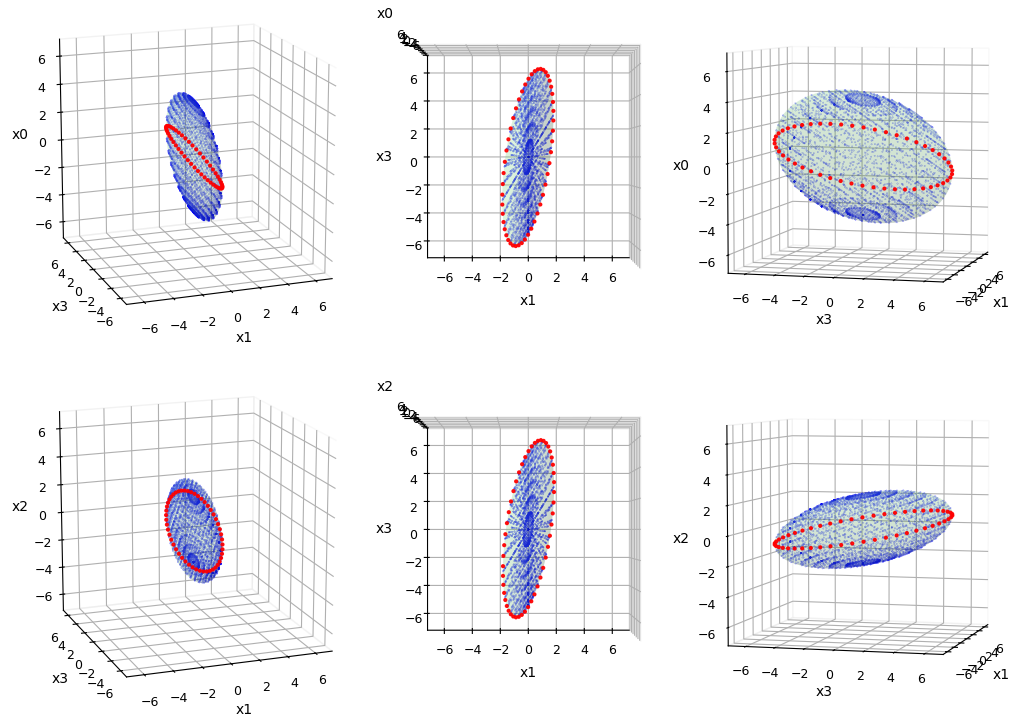
Now, you may ask: What about creating a transparent and continuous hull from tangential points computed on an angle-meshgrid? This is a variant of method 4A for 3-dim sub-spaces. Well, I have programmed this, too. Here you get the plot for a different filling pattern of the 𝕊³ and the hull in orange.

Or for another sub-space and another filling pattern:

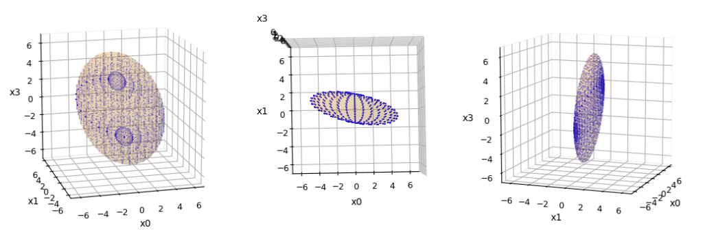
We can even add the tangential points (10,000; 100 per angle) with a decent transparency (here in red). Note that the points on the meshgrid also exhibit a pattern due to the filing of the 𝕊²-like intersection with the 𝕊³:

Nevertheless, the points never leave the ellipsoidal border indicated by the out-most data (blue points) of the original ellipsoid. The next plot shows a overlay of the tangential points only, without the continuous surface:

Conclusion

The orthogonal projections of ellipsoids defined in a multidimensional Euclidean space down to lower dimensional sub-spaces are controlled by relatively complicated mathematical relations. In this post we have shown with the help of numerical and graphical means that the formulas which we have derived in previous posts really give us the right predictions for projections of an ellipsoid from a 4-dimensional space to 3- and 2-dimensional sub-spaces. In all cases the hull of the projection image of the ellipsoid was computed correctly.

In the next post I will break down an ellipsoid from a really high-dimensional space down to 3- and 2- dimensional sub-spaces and apply the same tools as above to visualize the results. In this experiment we will create ellipsoidal hulls for data of a limited ellipsoidal core of a Multivariate Normal Distribution.