Compute confidence ellipses – I – simple method based on the Pearson correlation coefficient

This post was motivated by a publication of Carsten Schelp [1]. Actually, a long time ago. I used his results in 2021, when I had to plot confidence ellipses during the analysis of statistical (multivariate) vector distributions produced a Machine Learning algorithm. So, all acknowledgements belong to Schelp’s work. However, his ideas have also triggered some of my own efforts to look deeper into properties both of Bivariate [BVD] and Multivariate Normal Distributions [MVDs].

In this post I want to show how Schelp’s suggestion regarding confidence ellipses relate to my own reflections on BVDs. Actually, we have stumbled about Schelp’s results already in a previous post in this blog – where we used the covariance matrix of a standardized BVD as an example for determining half-axes of a respective contour ellipse. While there are other methods available to construct confidence ellipses for two-dimensional distributions of correlated data, Schelp’s ideas are very easy to implement in Python programs. And, of course, confidence ellipses based on elements of a covariance matrix are particularly useful for the analysis of approximate BVD-distributions.

We work in a 2-dimensional Cartesian coordinate system [CCS]. We will combine a lot of results previously derived in this blog. The interested reader should meanwhile know how BVDs result from linear transformations of the product of two independent standardized Gaussian vector distributions. You should also know the involved matrices controlling the probability density function of a BVD, the definition of contour ellipses via the so called Mahalanobis distance and the general definition of ellipses via symmetric, invertible and positive-definite (2×2)-matrices. A series of posts in this blog will give you the necessary information and formulas. In the last section you find respective links. Below, I will only give a brief summary.

Quadratic forms and ellipses

In post [2] I have shown that the coefficients of a quadratic form for the definition of an ellipse centered in our CCS can be interpreted as the elements of an invertible, positive-definite and symmetric matrix:

\[ \pmb{\operatorname{A}}_q \:=\: \begin{pmatrix} \alpha & \beta / 2 \\ \beta / 2 & \gamma \end{pmatrix} \,\,, \tag{1} \]

\[ \pmb{v}_E^T \circ \pmb{\operatorname{A}}_q \circ \pmb{v}_E \:=\: 1 \,. \tag{2} \]

v_E are vectors reaching from the CCS-origin to points on the ellipse, which due to a correlation of the coordinates will be rotated by an angle Φ against the CCS-axes. We have seen that the eigenvalues of A_q define the lengths of the half-axes of the corresponding ellipse via the following relations

\[ \begin{align} h_1 \:=\: {1 \over \sqrt{\lambda_1^{\phantom{1}} } } \,, \quad h_2 \:=\: {1 \over \sqrt{\lambda_2^{\phantom{1}} } } \,, \tag{3} \end{align} \]

\[ \begin{align} \lambda_1 \,&=\, {1\over 2}\, \left[\, (\,\alpha\,+\,\gamma\,) \,-\, \left[\, \beta^2 \,+\, \left(\,\gamma \,-\,\alpha \,\right)^2\, \right]^{1/2} \, \right] \,, \tag{4} \\[10pt] \lambda_2 \,&=\, {1\over 2}\, \left[\, (\,\alpha\,+\,\gamma\,) \,+\, \left[\, \beta^2 \,+\, \left(\,\gamma \,-\,\alpha \,\right)^2\, \right]^{1/2} \, \right] \,.\tag{5} \end{align} \]

λ₁ always gives us the longer half-axis. The rotation angle of the ellipse is also given by the matrix elements. We have clarified in [2] that we can always assume the longer axis to be oriented along the CCS’ x-axes ahead of a due rotation by Φ if we follow some rules for the angle

\[ \begin{align} \gamma \, – \, \alpha \,\ge\, 0, \,\, \beta \,\lt\, 0, \,\, \rho \,\gt \,0 \,\,& : \,\,\quad \phi \,= \, \psi , \quad \quad \quad \,\,(\psi \gt 0) \,, \,\, \quad \quad 0 \,\le\, \phi \,\le\, \pi/4 \,, \\[10pt] \gamma \, – \, \alpha \,\ge\, 0, \,\, \beta \,\gt\, 0, \,\, \rho \,\lt \,0 \,\,& : \,\,\quad \phi \,= \, \psi , \quad \quad \quad \,\,(\psi \lt 0) \,, \,\, -\, \pi/4 \,\le\, \phi \le \, 0 \,, \\[10pt] \gamma \, – \, \alpha \,\le\, 0, \,\, \beta \,\lt\, 0, \,\, \rho \,\gt \,0 \,\,& : \,\,\quad \phi \,= \, \pi/2 \,-\, \psi , \,\,(\psi \gt 0) \,, \,\,\quad \pi/4 \,\le\, \phi \,\le\, \pi/2 \,, \\[10pt] \gamma \, – \, \alpha \,\le\, 0, \,\, \beta \,\gt\, 0, \,\, \rho \,\lt \,0 \,\,& : \,\,\quad \phi \,= \, \pi/2 \,-\, \psi , \,\,(\psi \lt 0) \,, \,\, \quad \pi/2 \,\le\, \phi \le \, 3 \,\pi/4 \,,\ \end{align} \tag{6} \]

where we have used a helper angle ψ

\[ \begin{align} \psi \::&=\:\, {1 \over 2} \operatorname{arcsin}\left( {-\, \beta \over \left[ \beta^2 \, +\, \left( \gamma \,-\, \alpha \right)^2 \, \right]^{1/2} } \right) \,, \\[10pt] -\pi/2 \,& \le\, \psi \,\le\,\pi/2 \,. \end{align}\tag{7} \]

For more details see a respective table and its derivation in [2].

Relation to the central matrices which control a BVD

The 2-dim probability density function of a BVD (centered in the CCS) is controlled by a variance-covariance matrix. It couples the original independent and standardized Gaussians in x and y-direction during a linear transformation of their product (see [3]). v is a position vectors to a point in the 2-dim CCS.

\[ \mbox{centered CCS :} \quad g_{2c}(x, y) \,=\, {1 \over 2 \pi \, \sigma_x \, \sigma_y } {1 \over { \sqrt{\, 1\,-\, \rho^2}} } \operatorname{exp} \left( – {1\over2} \, {\pmb{v}}^{\operatorname{T}} \bullet \, \pmb{\Sigma}^{-1} \bullet {\pmb{v}} \, \right) \,. \tag{8} \]

The interesting point is that the inverse (Σ^-1) of the BVD’s variance-covariance matrix Σ

\[ \begin{align} &\pmb{\Sigma} \,=\, \begin{pmatrix} \sigma_x^2 &\rho\, \sigma_x\sigma_y \\ \rho\, \sigma_x\sigma_y & \sigma_y^2 \end{pmatrix} \,, \tag{9} \\[10pt] &\pmb{\Sigma}^{-1} \,=\, {1 \over \sigma_x^2\, \sigma_y^2\, \left( 1\,-\, \rho^2\right) } \, \begin{pmatrix} \sigma_y^2 &-\rho\, \sigma_x\sigma_y \\ -\rho\, \sigma_x\sigma_y & \sigma_x^2 \end{pmatrix} \,, \tag{10} \\[10pt] & \pmb{\Sigma} \bullet \pmb{\Sigma}^{-1} = \mathbf I_n \,. \tag{11} \end{align} \]

defines contour ellipses of the probability density function of a BVD. σ_x and σ_y are the standard deviations of a BVD’s marginal distributions along the coordinate axes. ρ is the respective Pearson correlation coefficient. The following equation defines an ellipse for a given value of the Mahalanobis distance d_m

\[ \begin{align} {\pmb{v}}^T \bullet \, \pmb{\Sigma}^{-1} \bullet {\pmb{v}} \,:=\, \left(d_m\right)^2\,, \tag{12} \\[10pt] d_m \,:=\, \sqrt{ \, {\pmb{v}}^{T^{\phantom{A}}} \bullet \, \pmb{\Sigma}^{-1} \bullet {\pmb{v}} } \,. \tag{13} \end{align} \]

Formally, we can combine d_m with the sigmas in a modified matrix Σ^-1_m to get an equation equivalent to (2).

\[ \begin{align} {\pmb{v}}^T \bullet \, \pmb{\Sigma}^{-1}_m \bullet {\pmb{v}} \:=\, 1 \,. \tag{14} \ \end{align} \]

We then can associate the elements of Σ^-1_m (of a BVD) with those of a general matrix A_q :

\[ \begin{align} \alpha \, &= \, {1 \over d_m^2 \, \sigma_x^ 2 \, \left( 1 \,-\, \rho^ 2 \right) } \,, \\[10pt] \beta \, & = \, { -\, 2\, \rho \over (d_m \, \sigma_x) \, (d_m \, \sigma_y) \, \left( 1 \,-\, \rho^ 2 \right) } \,, \\[10pt] \gamma \, &= \, {1 \over d_m^2 \, \sigma_y^ 2 \, \left( 1 \,-\, \rho^ 2 \right) } \,. \tag{15} \end{align} \]

We know already (see e.g. [3] and [4]) that a decomposition of the symmetric Σ^-1_m , e.g. an eigendecomposition, will give us a matrix M

\[ \begin{align} \operatorname{ \pmb{\Sigma}}_m \:&=\: \operatorname{\pmb{M}} \bullet \, \operatorname{\pmb{M}}^T \,, \\[10pt] \operatorname{ \pmb{\Sigma}}_m^{-1} \:&=\: \left[\operatorname{\pmb{M}}^{-1}\right]^T \bullet \operatorname{\pmb{M}}^{-1} \,. \\[10pt] \end{align} \tag{16} \]

by which we can create vectors v_E defining our the ellipse via a linear transformation of vectors defining a unit circle.

\[ \begin{align} \pmb{z} \, &=\, \begin{pmatrix} \cos \theta \\ \sin \theta \end{pmatrix} \,, \\[10pt] \pmb{v}_E \, &= \, \operatorname{\pmb{M}} \bullet \, \pmb{z}, \, \quad \pmb{z} \,=\, \operatorname{\pmb{M}}^{-1} \bullet \pmb{v}_E \,. \end{align} \tag{16}\]

The vectors z define circle contours of the product of two independent standardized and centered Gaussians in x– and y-direction at a distance d = 1 from the origin. For more information on how a BVD is created from a combination of independent Gaussians see [2].

Ellipses for two dimensional correlated data samples

For a given sample of data points, whose x- and y-coordinates are correlated, in two dimensions we can under normal conditions compute a symmetric covariance matrix. As long as this matrix is invertible and has positive eigenvalues we can interpret it as a control matrix for an assumed BVD – and produce BVD contour ellipses (dependent on given Mahalanobis distance values) for this BVD.

Such ellipses may help to understand the real data distribution and its similarity with or difference from a respective BVD better.

Use of a standardized BVD to construct a confidence ellipse

The transformation matrix M which generates a BVD also creates the BVD’s marginal distributions along the coordinate axes. These marginal Gaussian distributions have characteristic standard deviations σ_x and σ_y.

It is, of course, possible to perform a scaling of such a given BVD along the CCS-axes such that the marginal Gaussians get standardized, i.e. such that we get σ_x = 1 and σ_y = 1. The required scaling is done by diagonal matrices – using 1/σ_x– and 1/σ_y -factors on its diagonal. The sigma-values are derived from a computed covariance matrix.

The nice thing about scaling operations (diagonal matrices) is that we can switch the position of the respective matrices in a series of linear transformations without causing trouble. For the simple construction of a confidence ellipse, it is therefore helpful

to first work with a standardized distribution achieved by scaling with 1/σ_x– and 1/σ_y -factors of a diagonal matrix,
to then compute an elementary ellipse based on the covariance matrix of a standardized BVD,
and afterward to compensate for the previous scaling again by stretching the data along the x– and y-axes, again, with the help of another diagonal matrix, now containing σ_x– and σ_y -factors.

Mathematically: During the construction of a contour ellipse with a matrix M from unit circle vectors, we apply a unit matrix, split it into two parts – the first one standardizing by scaling with 1/σ_x, 1/σ_y – and the second part stretching by σ_x, σ_y, again – and rearrange the order of operations. (To account for confidence levels we apply an additional stretching by d_m in the end.)

So, let us first set

\[ d_m \,=\, 1\,, \quad \sigma_x \,=\, 1\,, \quad \sigma_y \,=\, 1\ \tag{17} \]

in our matrices Σ , Σ^-1 to get modified versions Σ_S , [Σ_S]^-1. The respective modified version M_S (of M) produces stretching and rotation effects due to the correlation ρ ≠ 0 when applied to unit circle vectors. The modified matrices look like

\[ \begin{align} &\pmb{\Sigma}_S \,=\, \begin{pmatrix} 1 &\rho \\ \rho & 1 \end{pmatrix} \,, \tag{18} \\[10pt] &\pmb{\Sigma}_S^{-1} \,=\, {1 \over \left( 1\,-\, \rho^2\right) } \, \begin{pmatrix} 1 &-\rho \\ -\rho\ & 1\end{pmatrix} \,. \tag{19} \\[10pt] &\alpha_S \,=\, 1\,, \quad \beta_S \,=\, -2 \,\rho\,, \quad \gamma_S \,=\, 1 \,. \end{align} \]

A quick calculation for the elements α_S, β_S and γ_S with eqs. (3) and (4) gives us the properties for a respective basic ellipse – stretched and rotated due to correlation:

\[ \begin{align} \lambda_{S1} \, &= \, {1\over (1 \,+\, |\rho| ) } \,, \quad h_{S1} \,=\, \sqrt{ \, 1 \, +\, |\rho|^{\phantom{1}} \, } \,, \tag{20} \\[10pt] \lambda_{S2} \, &= \, {1\over (1 \,- \, |\rho| ) } \,, \quad h_{S2} \,=\, \sqrt{ \, 1 \, – \, |\rho|^{\phantom{1}} \, } \,.\tag{21} \\[10pt] \psi_S \, &= \, \pm \,\pi / 4 \,. \tag{22} \end{align} \]

The angle of rotation of this ellipse against the CCS is a bit of a mess. To get it correctly, we have to take into account a later potential stretching with σ_x * d_m, σ_y * d_m to do the right thing for our construction of the confidence ellipses, namely to achieve consistency with our conditions (6).

Eventual recipe

Going through all conditions systematically shows that we do everything correctly when we define the half-axes in x– and y-direction ahead of rotation by

\[ \begin{align} \lambda_{S,x} \, &= \, {1\over (1 \,+\, \rho ) } \,, \quad h_{S,x} \,=\, \sqrt{ \, 1 \, +\, \rho^{\phantom{1}} \, } \,, \tag{23} \\[10pt] \lambda_{S,y} \, &= \, {1\over (1 \,- \, \rho ) } \,, \quad h_{S,y} \,=\, \sqrt{ \, 1 \, – \, \rho^{\phantom{1}} \, } \,.\tag{24} \\[10pt] \phi_S \,&=\, \pi/4 \,. \tag{25} \end{align} \]

Note that we now allow the sign of ρ to change! This shifts the longer axis into y-direction for negative ρ. And we specify Φ_S instead of ψ.

This simple setting accounts for the correct orientations when we afterward stretch the coordinates with some factors σ_x * d_m, σ_y * d_m – and thereby create one of the possible cases listed in (6). The resulting angle of the longer axis then actually turns into those right angle regions, which the conditions (6) require.

You can prove this by some simple sketches and analyzing what effects a stretching with different σ_x– and σ_y-values and the respective difference (γ_S – α_S) causes. But, we can also make some quick tests with a Python-program, too. See below.

I summarize the steps to create a contour or confidence ellipse for a given Mahalanobis distance d_m fulfilling eqs. (12) or (14) for a given sufficiently large sample of data points of an approximate BVD:

Recipe to construct a contour ellipse for a given Mahalanobis distance d_m

Step 1: Determine the center of your distribution and a respective vector and move the distribution by a respective vector translation to become a centered distribution in your CCS.
Step 2: Numerically determine the respective variance-covariance matrix. (Numpy as well as other libraries have functions to do this for you). Determine the Pearson coefficient ρ.
Step 3: Use eqs. (23) to (25) to create an ellipse with half-axis sqrt(1 + ρ) in x-direction and sqrt(1 – ρ) in y-direction. Rotate this ellipse by Φ = π/4 in anti-clockwise direction.
Step 4: Rescale your vector-components in x-direction by d_m* σ_x and in y-direction by d_m* σ_y.

Some difference to Schelp’s recipe – confidence levels

Regarding confidence ellipses there is a major difference to Schelp’s recipe. He in early versions of his article had claimed that you should rescale by integer values of d_m to reach typical confidence levels according to the 68-95-99.7 rule. Unfortunately, this is not correct. And Schelp himself has criticized this later on. We can do somewhat better, already:

In [5] we have shown that cumulative probabilities P for finding BVD data-points within a d_m – ellipse are related to d_m by

\[ d_m \:=\: d_m\left(P\right) \:=\: \sqrt{ \,-\, 2 \, \ln \left(\, 1 \,-\, P\, \right) } \,. \tag{26}\]

In particular, we have:

P = 0.50 : d_m = 1.177 || P = 0.70 : d_m = 1.552 || P = 0.75 : d_m = 1.665 ||
P = 0.80 : d_m = 1.794 || P = 0.85 : d_m = 1.948 || P = 0.90 : d_m = 2.146 ||
P = 0.95 : d_m = 2.448 || P = 0.99 : d_m = 3.035.

Simple tests with statistical vectors of a BVD

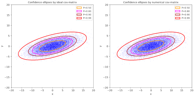
The following plots cover the four cases distinguished in the relations and conditions of (6) above. I have created “centered” BVDs with 16000 data points. Despite the big number the center of the distribution does not exactly coincide with the origin of the CCS. Also numerically covariance matrices do not fully reproduce the data of the covariance matrix used to create the BVD points. The deviations are in the region of some percent.

The left sub-plot for every case shows confidence ellipses computed from the ideal covariance matrix used to generate the BVD data-points. The right sub-plot, instead, shows the ellipses computed from numerically centering the distribution and creating the ellipses from a numerically determined covariance matrix (based on the vectors to the data points).

The ellipses themselves were created with functions of the “matplotlib.transforms” module.


...    
    ellipse = Ellipse((0, 0), width=ell_radius_x * 2, height=ell_radius_y * 2,
                      facecolor=facecolor, lw=linew, **kwargs)
....
    transf = transforms.Affine2D() \
        .rotate_deg(45) \
        .scale(scale_x, scale_y) \
        .translate(mean_x, mean_y)
....
    ellipse.set_transform(transf + ax.transData)
....

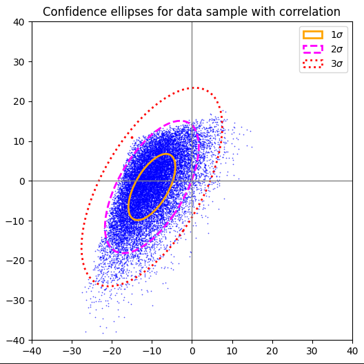
Plot 1 / case 1
ρ > 0, (γ – α) ≥ 0, 0 ≤ Φ ≤ π/4, cov = Σ = [[30,+7] [+7,5]], positive correlation
numerical data :
cov = [[30.31708014, 7.06327008], [ 7.06327008, 5.01330231]]
mean_x = -0.01765997032310763, mean_y = 0.009496864248879522

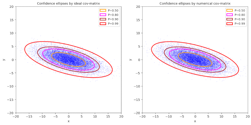
Plot 2 / case 2
ρ < 0, (γ – α) ≥ 0, -π/4 ≤ Φ ≤ 0, cov = Σ = [[30,-7] [-7,5]], negative correlation
numerical data:
cov = [[30.08681948, -7.02386134], [-7.02386134, 5.01516656]]
mean_x = -0.09396637122815052, mean_y = 0.022298783828165903

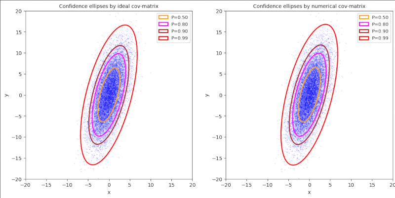
Plot 3 / case 3
ρ > 0, (γ – α) ≤ 0, π/4 ≤ Φ ≤ π/2, cov = Σ = [[5,+7] [+7,30]], positive correlation
cov = [[ 4.98127006, 6.95301673], [ 6.95301673, 30.12507367]]
mean_x = 0.032945621849379686, mean_y = 0.10092847791754798

Plot 4 / case 4
ρ < 0, (γ – α) ≤ 0, π/2 ≤ Φ ≤ 3π/4, cov = Σ = [[5,-7] [-7,30]], negative correlation
numerical data :
cov =[[ 5.10239329, -7.04155687], [-7.04155687, 30.28164018]]
mean_x = -0.008791792672444138 , mean_y = -0.03660849288658889

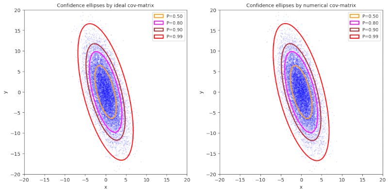
The nice thing is that Schelp’s method adjusts the correct orientation confidence ellipses automatically.

Tests for samples of other 2-dim data point distributions with correlated coordinates

Just to have some fun: The following plots show confidence ellipses for statistically generated data point distributions in two dimensions, for which have enforced some correlation of the x– and y-coordinates. The basic distributions in each coordinate direction do not follow normal Gaussians. They are not even symmetric. The plotting of confidence ellipses supports the visual impression how different the distributions are from BVDs.

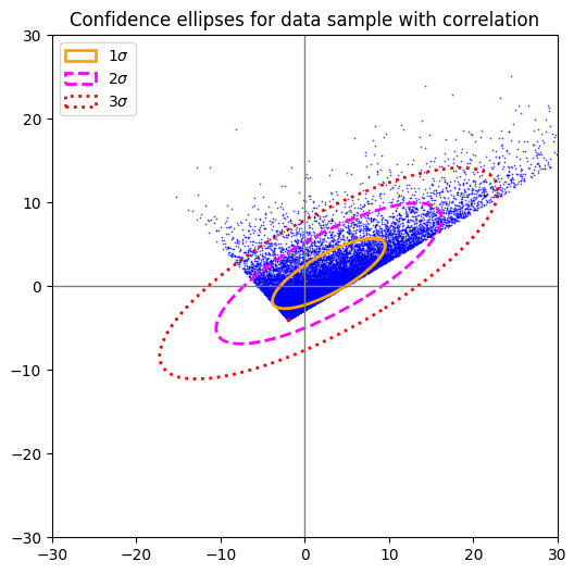
Plot for 2-dim Rayleig-distribution after linear and correlating transformation
Just to have some fun and to show that we can plot confidence ellipses also for other 2-dimensional distributions than normal ones, I have generated a linearly transformed 2-dim distribution where the data points in both coordinate direction followed a Rayleigh distribution before a linear and correlating matrix was applied. We see clearly that the underlying distribution is not a BVD, not even an approximate one.

Plot for 2-dim exponential distribution after linear and correlating transformation
Here a transformed exponential distribution in two directions

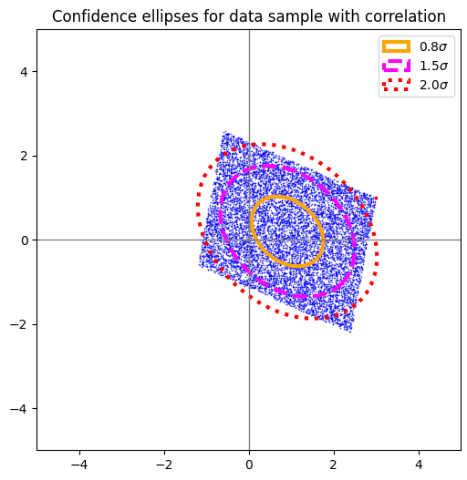
Plot for 2-dim uniform distribution after linear and correlating transformation
The data in this case followed a uniform distribution in both coordinate directions before they were correlated by a linear transformation.

Conclusion

In this post I have reproduced the method of Carsten Schelp [1] to easily create confidence ellipses based on a variance-covariance matrix of a 2-dimensional data distribution. The required steps were motivated by previous results derived in this blog. This method makes of course most sense when applied to distributions which at least up to a certain distance approximate a Bivariate Normal Distribution. In such cases we can associate cumulative probability levels with certain values of the Mahalanobis distance. However, the method can also be applied to other 2-dimensional data distributions as long as they have a pronounced center. It then helps to make differences in comparison with BVDs clearly visible.

Links and literature

[1] Carsten Schelp, “An Alternative Way to Plot the Covariance Ellipse”,
https://carstenschelp.github.io/2018/09/14/Plot_Confidence_Ellipse_001.html

[2] R. Mönchmeyer, 2025, “Ellipses via matrix elements – I – basic derivations and formulas”,
https://machine-learning.anracom.com/2025/07/17/ellipses-via-matrix-elements-i-basic-derivations-and-formulas

[3] R. Mönchmeyer, 2025, “Bivariate normal distribution – derivation by linear transformation of a random vector of two independent Gaussians”,
https://machine-learning.anracom.com/2025/06/24/bivariate-normal-distribution-derivation-by-linear-transformation-of-random-vector-of-two-independent-gaussians

[4] R. Mönchmeyer, 2025, “Bivariate normal distribution – explicit reconstruction of a BVD random vector via Cholesky decomposition of the covariance matrix”,
https://machine-learning.anracom.com/2025/06/27/bivariate-normal-distribution-explicit-reconstruction-of-a-bvd-random-vector-via-cholesky-decomposition-of-the-covariance-matrix

[5] R. Mönchmeyer, 2025, “Bivariate Normal Distribution – integrated probability up to a given Mahalanobis distance, the Chi-squared distribution and confidence ellipses”,
https://machine-learning.anracom.com/2025/07/30/bivariate-normal-distribution-integrated-probability-up-to-a-given-mahalanobis-distance-the-chi-squared-distribution-and-confidence-ellipses