Ellipses are specific two-dimensional geometrical objects. They are of interest in many contexts – e.g. in physics, engineering and in cryptography. However, they also appear in statistics. For example, in the form of elliptic contour lines of Bivariate Normal Distributions [BVDs] and as elliptic contours of the projections of Multivariate Normal Distributions [MVDs] onto coordinate planes. Approximate BVDs/MVDs in turn often appear as input data of Machine Learning [ML] algorithms – or sometimes also as result data in latent spaces of neural networks.

This post discusses basic mathematical aspects of ellipses. My main objective is to explain the relation between geometrical properties of an ellipse and the elements of two special matrices which describe a (rotated) ellipse in different ways. These matrices are related to so called quadratic forms describing ellipses.

When we deal with data of statistical vector distributions, we regularly have to derive geometrical properties of contour and confidence ellipses from numerically calculated elements of a variance-covariance matrix. Another task is the calculation of the properties of an ellipse from the coefficients of its quadratic form. The results of this post can be helpful to solve such problems.

This post is a revised and extended version of thoughts and formulas which I have previously presented in a post of a sister blog on Linux topics. This post will show you how results, which you may find elsewhere, are derived from first principles. A special topic is the determination of the rotation angle of an ellipse from matrix elements. While other texts on the topic jump over related ambiguities, I have tried to present respective considerations as clearly as possible. In a second post I will give you numerical examples and show some plots. Other posts in this blog will apply the results to BVDs and MVDs.

We work in a 2-dimensional Cartesian coordinate system [CCS]. When I speak of vectors, I mean position-vectors from the origin of our chosen CCS to points somewhere in our 2-dimensional space. The components of such vectors have values that are equal to the (x,y)-coordinates of the points in our CCS. Required knowledge is some basic trigonometry and some Linear Algebra.

Related posts:

• Ellipses via matrix elements – II – numerical tests of formulas
• Cholesky decomposition of an ellipse-defining symmetric matrix
• Bivariate Normal Distribution – Mahalanobis distance and contour ellipses

Introduction

Geometrically, we describe ellipses in terms of their two perpendicular principal axes, focal points, ellipticity and rotation angles with respect to a CCS. Another aspect is:

Ellipsoids/ellipses can in general be defined and/or created by matrices operating on position vectors. The elements of such matrices are related to coefficients of quadratic polynomial expressions which control the coordinates of points on an elliptic curve. Such quadratic forms in turn describe ellipses as a specific type of conic sections.

Ellipses are typically rotated against the axes of the chosen CCS. The rotation angle of an ellipse’s longest axis against the x-coordinate axis reflects a specific correlation of the x– and y-components of vectors reaching from the origin of the CCS to points on the ellipse.

Questions about ellipses

There are five questions which I want to cover in this and a forthcoming post:

• What kind of matrices define 2-dimensional elliptic curves? How can we build such matrices from elementary vector operations – such as scaling/stretching and rotation? Vector operations applied to vectors of what, exactly?
• How do the matrix elements define the coordinates of points on a ellipse?
• How can one derive the lengths h₁, h₂ of the (perpendicular) principal axes of an ellipse from the elements of relevant matrices? In particular of symmetric matrices that correspond to quadratic forms?
• How do the eigen-decomposition or the Cholesky-decomposition of such a symmetric matrix fit into the picture?
• By which formula do the matrix elements provide the inclination angle of the ellipse’s primary axes? What about ambiguities coming from multiple solutions of trigonometric functions and/or from certain degrees of freedom when creating the ellipse?

Three defining matrices for centered ellipses

In this post we only regard ellipses whose centers coincide with the origin of a chosen CCS. We thereby get rid of boring constant terms in the equations we have to solve. We do not loose much of general validity by this step: Results of an off-center ellipse follow from applying a simple translation operation to the resulting vector data.

The longer principal axis of an ellipse may be inclined by some angle Φ against the x-axis of our CCS. If Φ = 0, we speak of an axis-parallel ellipse: The half-axes of such an ellipse are oriented in parallel to the coordinate axes of the CCS. The algebraic terms to describe such an ellipse with half-axes h₁ in x-direction and h₂ in y-direction should be familiar from school:

x_E and y_E are coordinates of points on the axis-parallel ellipse.

There are actually (at least) three important and different ways to define a centered and rotated ellipse by a matrix:

• Alternative 1: We define the (rotated) ellipse by a matrix A_E which results from the (matrix) product of two simpler matrices: A_E = R_Φ • D_E:
  D_E is a diagonal matrix and corresponds to a scaling operation applied to the components of vectors to points located on a centered unit circle. This leads to an axis-parallel ellipse. We will show that stretching a unit circle by D_E reproduces the standard definition formula (0.1) of an axis-parallel ellipse.
  R_Φ describes a subsequent rotation by an angle Φ. A_E summarizes these geometrical operations in a compact form.
• Alternative 2: We define a (rotated) ellipse by a matrix A_q which acts on a vector v such that we get a polynomial equation with quadratic terms in the vector components (v^T • A_q • v; see below). I.e., matrix A_q gives us a so called quadratic form. Geometrically interpreted, a quadratic form describes an ellipse as a special case of a conic section. The coefficients of the polynomial and the elements of the matrix must, of course, fulfill some particular properties.
• Alternative 3: From the inverse of A_q one can derive a matrix K_ch via a Cholesky decomposition. This matrix can also be applied to vectors on a unit circle to create an ellipse

Note that Alternative 1 comes with an ambiguity besides the choice of an angle : The creator of an ellipse (and of a respective matrix A_E) has the freedom to decide which half-axis shall become the longer one. Formally, we associate h₁ with the half-axis of the original axis-parallel ellipse in x-direction, and h₂ with the half-axis of the original axis-parallel ellipse in y-direction. This gives rise to two situations:

The differences will occupy us a bit in this text.

Major mathematical steps

While it is relatively simple to derive the matrix elements from known values of h₁, h₂ and Φ, it is a bit harder to derive an ellipse’s properties from the elements of the two defining matrices A_E and A_q. This, however, is our main objective. We will cover both matrices.

Our approach will comprise seven main steps, each of which means solving a specific mathematical task:

1. Step 1: We derive the dependency of the elements (a, b, c, d) of A_E on the geometrical properties of a corresponding ellipse: A_E = A_E (h₁, h₂, Φ) .
2. Step 2: We use A_E to create a unique quadratic form which defines the ellipse.
3. Step 3: We compare the coefficients derived in step 2 with the coefficients of a general quadratic equation mediated by a symmetric matrix A_q: v^T • A_q • v = 1.
   We then establish relations of the A_q elements α, β, γ with h₁, h₂, Φ : α=α(h₁,h₂,Φ), β=β(h₁,h₂,Φ), γ=γ(h₁,h₂,Φ).
4. Step 4: We invert the results of step 3 to get relations of the form
   h₁=h₁(α,β,γ), h₂=h₂(α,β,γ), Φ=Φ(α,β,γ) and
   h₁=h₁(a,b,c,d), h₂=h₂(a,b,c,d), Φ=Φ(a,b,c,d).
5. Step 5: We establish relations of h₁, h₂, Φ with the the eigenvalues λ₁, λ₂ and respective eigenvectors of A_q.
6. Step 6: We briefly discuss the creation of an ellipse by a matrix K_ch coming from the Cholesky decomposition of A_q‘s inverse matrix.
7. Step 7: We discuss various cases and conditions giving us different distinct formulas for the rotation angle Φ = Φ (λ₁, λ₂, α, β, γ) .

For many practical purposes steps 5 and 7 are of special interest.

Step 1: Matrix A_E for the creation of a centered and rotated ellipse – scaling of a unit circle followed by a rotation

Our starting point is a unit circle C whose center coincides with the origin of our CCS. The components of vectors v_c from the origin to points on the circle C fulfill the following conditions:

and

We define an ellipse E(h₁, h₂) (having half-axes h₁ and h₂) by the application of two linear operations to the vectors v_c:

D_E is a diagonal matrix which describes a stretching of the circle along the CCS-axes, and R_Φ is an orthogonal rotation matrix. “○” symbolizes the standard matrix multiplication.

The stretching (or scaling) of the vector-components is done by matrix D_E :

We will see in a minute that the application of D_E on vectors v_c indeed is equivalent to the standard definition (E) of a centered, axis-parallel ellipse. Therefore, the elements h₁, h₂ of D_E define the lengths of the principal axes of the yet un-rotated ellipse: h₁ is half of the ellipse’s diameter in x-direction, h₂ is half of the diameter in y-direction.

The subsequent rotation by an angle Φ against the x-axis of the CCS is done by a standard rotation matrix R_Φ:

Combining both operations results in a matrix A_E with elements ((a, b), (c, d)):

Note:

Remember:

We introduce new variables λ₁ and λ₂

and get

The mathematical meanings of λ₁ and λ₂ will become clearer in a later section. The determinant of matrix A_E is given by

h₁ and h₂ refer to the lengths of the principal axes of the ellipse. h₁ and h₂ have positive values by definition. Therefore:

We have succeeded with step 1: We have defined an ellipse via an invertible (and also positive definite) matrix A_E, whose elements are directly based on geometrical properties.

But as said: Often an ellipse is described by a quadratic form. As a next step we derive such a quadratic equation first for an axis-parallel ellipse. Afterward we move on to a general rotated ellipse. This will in turn define another very useful matrix A_q.

Quadratic form describing a centered, un-rotated, axis-parallel ellipse

let us look at an ellipse which results from applying our scaling matrix D_E to our unit circle C. I.e., the rotation matrix is assumed to be just the identity matrix:

We need an expression in terms of (x_E, y_E). To get quadratic terms of vector components it helps to invoke a scalar product. The scalar product of a vector with itself gives us the squared length of a vector. In our case the norm of the inversely scaled vectors has to fulfill:

This directly results in:

This, obviously, is the standard definition (E) of an (axis-parallel) eclipse. We replace the denominators to get a convenient quadratic form:

If someone had given us the quadratic form more generally with coefficients α, β and γ

we could have directly related these coefficients with the geometrical properties of our axis-parallel ellipse:

A first success: We can derive h₁, h₂ and Φ from the coefficients of the (reduced) quadratic form. But an axis-parallel ellipse is a simple case. Things get more difficult for a general rotated ellipse. Then we have to care about the mixing term with β ≠ 0.

Step 2: Quadratic form defining a general centered and rotated ellipse

We turn to step 2, now. To get a quadratic polynomial for a rotated ellipse, we use the trick from the last section once again. We apply a full back-transformation [A_E]^-1 to vectors v_E of a general ellipse:

This leads to equations for the elements of matrix A_E :

The rotation included in A_E has obviously lead to a mixing of the vector components (x_E, y_E) in the polynomial: The coefficient for x_E y_E is different from zero in the general, non-trivial case.

Step 3: Quadratic form of an ellipse: Definition by a symmetric, invertible (2×2)-matrix A_q

We rewrite our polynomial equation again with general coefficients α, β and γ:

With the help of a symmetric (2×2)-matrix A_q, the quadratic polynomial can be reformulated:

with

Of course, the elements of such a matrix must fulfill certain conditions to really define an ellipse. A comparison with eq. (27) shows

This in turn means

With

it follows that

The elements of matrix A_q are intimately related to the ellipse’s geometrical data, but in a somewhat convoluted way. We have to explore these relations in more detail.

With the help of the elements of A_E we can also show that det(A_q) > 0:

To describe an ellipse A_q must be an invertible matrix, too. At least for standard conditions (h₁ >0, h₂ > 0). Furthermore, A_q is obviously symmetric and thus its own transposed matrix. Eq. (39) can be regarded as a necessary condition for any symmetric matrix that shall describe an ellipse! We will see later later that A_q must in addition be a positive-definite matrix.

By the way: Eq. (39) tells us that α and γ must have the same sign – and β must fulfill a condition:

We will derive further conditions later on.

Success for step 3: We have written down A_q‘s elements α, β, γ as some relatively simple functions of a, b, c, d and thus of h₁, h₂ and Φ. We now focus on the question of how we can express h₁, h₂ and Φ as functions of either (a, b, c, d) or (α, β, γ).

How to derive h₁, h₂ and Φ from the elements of A_E or A_q in the general case?

Let us assume we have (numerical) data for the coefficients of the quadratic form and thus of matrix A_q. Then we may want to calculate values for the length of the principal axes and the rotation angle Φ of the corresponding ellipse. There are two ways to derive respective formulas:

1. Approach 1: We use trigonometric relations to directly solve a respective equation system. This corresponds to step 4.
2. Approach 2: We use an eigenvector decomposition of A_q. This will help us to solve the tasks of step 5.

We study both paths below.

Step 4.1: Derivation of h₁, h₂ and Φ from the elements of matrix A_q via trigonometric relations

Helpful trigonometric relations are:

We do not make any assumptions, yet, about the difference h₁ – h₂. Remember, that our ellipse could have been created with either inequality of its half-axes. See the alternatives in the inequalities (C).

By combining the above relations (36) to (38) for the elements of A_q we find

Eqs. (44) and (45) are key-relations! We have to treat them carefully.

By squaring and adding the last two equations we further get

From eq. (46.1) together with with ineq. {39.1} we find that the following conditions must be fulfilled at the same time

to guarantee that both axes have a positive length. These are conditions which correspond to the invertibility and the positive-definiteness of A_q.

Two basic cases we have to distinguish

We are now confronted with our two elementary cases (C) – depending on how we had chosen to scale the half-axes of the original axis-parallel ellipse and the sub-sequent rotation angle Φ.

Case 1: λ₂ ≥ λ₁

In this case we would have started our construction of our ellipse with h₁ ≥ h₂. Let us call the resulting ellipse E_1>2. Then:

with, obviously, λ₂ ≥ λ₁. We define the following helper angle ψ, whose sign only depends on β

Note that this reduces the solution space of eq. (45), because by definition of the arcsin-function we have:

For the rotation angle Φ we, therefore, get two potentially valid results of eq. (45)

This raises the questions: What conditions let us decide between the two options?

Well we should not forget eq. (44). Let us consider the example of β < 0 and at the same time (γ – α) ≥ 0. Then ψ is positive. But Φ must fulfill two conditions, namely (44) and (45) :

For the given conditions this restricts us to the solution given by (51.1).

This example shows that a proper choice depends on all elements of matrix α, β, γ – and a fulfillment of both eqs. (44) and (45). See a later section below for a proper treatment of all possible cases. Such a distinction of multiple solutions for the rotation angle is necessary, when you want to reconstruct ellipses by numerical methods from a given matrix A_q.

Case 2: λ₂ < λ₁

Some matrices may describe ellipses whose half-axis in y-direction had been longer than its half-axis in x-direction, ahead of rotation. Let us call such an ellipse E_2>1. Then λ₁ and λ₂ would switch their role:

Note that a rotation of such an ellipse by Φ = – (π/2 – ψ) would, for the same values α, β , γ ), give us the same ellipse as case 1!

Eq.(45), once again, indicates that we must choose between two alternatives

Let us again consider an example, namely for β < 0, (γ – α) ≥ 0. By analyzing the two conditions (44) and (45) we get for the smallest value of |Φ|:

This fits solution (52.2) .

Remaining ambiguities?

Although we have in principle succeeded with parts of step 4, the remaining choices leave us a bit skeptical for the time being. It seems that we can impose restrictive conditions on the range of Φ; this may select one of two possible solutions regarding the sine-function. However, the natural natural ambiguity described in (C) and which led us two the distinguished two cases 1 and 2 could not be resolved by a comparison of A_q with A_E alone.

We will come back to this point in a special section below, where we will summarize all possible scenarios. We will eventually see that whenever we need to create a proper ellipse given by a symmetric, positive definite matrix A_q we can safely cling to Case 1 (λ₂ ≥ λ₁), for which we only must distinguish 4 sub-cases depending on the values of β and (γ – α).

Example: Standardized BVD

A simple example for a matrix A_q would be one that appears in the context of a standardized (!) Bivariate Normal Distribution [BVD] with some correlation imposed onto the statistical variables:

With ρ > 0 being the Pearson correlation coefficient. For this case we get the following result for the half axes of a respective ellipse and the rotation angle Φ:

Hint: These are very useful equations for a numerical reconstruction of contour ellipses of a BVD. I will describe this in more detail in other posts of this blog.

Step 4.2: Derivation of h₁, h₂ and Φ from the elements of A_E via trigonometric relations

Let us quickly look at the relation of the elements of matrix A_E with geometric properties of a respective ellipse. We set

This gives us

and

We rearrange terms and get:

So far, so good. But the equations are a bit hard to tackle. Let us, therefore, define some further variables before we add and subtract the first two of the above equations:

Adding two of the equations with the sin(2Φ) and cos(2Φ) above and using the third equation results in:

Again, we must distinguish 2 cases:

Case 1: ε₁ > ε₂

In terms of the matrix elements a, b, c, d:

Who said that life had to be easy? I leave it to the reader to show with the help of eq.(31) that this is identical to eqs. (48) and (49).

Case 2: ε₂ > ε₁

It is relatively easy to prove:

We thus can rewrite eq. (31) as

Determination of the inclination angle Φ via elements of A_E

For the determination of the angle Φ we use:

We choose

and get:

Note: All in all there are four different solutions. The reason is that we alternatively could have requested λ₂ ≥ λ₁ or λ₁ ≥ λ₂, and in addition chosen a different angle. Again, we find ambiguities due to a selection of the considered principal axis and rotational symmetries. See a later section for a proper distinction between all reasonable cases.

Step 5: 2nd way to a solution for h₁, h₂ and Φ via eigendecomposition of A_q

We now turn to step 5. For our second way of deriving formulas for h₁, h₂ and Φ we use some Linear Algebra. Above we have written down a symmetric, positive-definite matrix A_q describing an operation on the position vectors of points on our rotated ellipse:

From Linear Algebra we know that every symmetric, real-valued and positive definite matrix can be decomposed into a product of orthogonal matrices O, O^T and a diagonal matrix. This reflects the so called eigendecomposition of a symmetric matrix:

with

The elements λ_u and λ_d are eigenvalues of both D_diag and A_q. Reason:
Orthogonal matrices do not change eigenvalues of a transformed matrix. So, the diagonal elements of D_diag are the eigenvalues of A_q, too. Linear Algebra also tells us that the columns of the matrix O are given by the components of the normalized eigenvectors of A_q. (The order of the eigenvalues along the diagonal is not pre-defined. Only by convention one would arrange them downwards in increasing order.)

We can interpret O as a rotation matrix R_Φ for some angle Φ:

The whole operation tells us a simple truth, which we are already familiar with:

By our construction procedure for a rotated ellipse we know that a (rotated) CCS exists, in which the ellipse can be described as the result of a scaling operation (along the coordinate axes of the rotated CCS) applied to a unit circle. (This CCS is, of course, rotated by an angle Φ against our working CCS in which the ellipse appears rotated.)

Above we had found

With our matrices R_Φ and the scaling matrix D_E we rewrite this as

A rearrangement tells us:

Now, we remember that a diagonal matrix is its own transposed matrix and that the inverse of an orthogonal matrix (rotation) is its transposed matrix:

Comparing with (857) we find:

We therefore may identify the eigenvalues as some familiar terms

The eigenvalues λ_u and λ_d of our symmetric matrix A_q are just our parameters λ₁ and λ₂. It is really noteworthy that the half-axes of the ellipse are given by the reciprocate value of the square root of the matrix’ eigenvalues:

Mathematically, a lengthy calculation to solve the eigenvalue-problem indeed reveals that the two eigenvalues of a symmetric matrix A_q with the elements α, β and γ have the following form:

I have used different indices here because of the following reason:

It is a priori not clear which of the eigenvalues has to be identified with the upper and lower elements of the central matrix D_diag. This reflects the already familiar ambiguity in how the ellipse was oriented before rotation and the resulting problem of finding a proper rotation angle from the eigendecomposition. See a later section for a solution.

Side remark: You can derive the results (94) to (96) a bit easier with solving the so called “characteristic equation” of the matrix. For more details see e.g.:
Eigenvalues and eigenvector of a positive-definite, real valued and symmetric matrix

Our result, of course, is consistent with what we have found above by solving respective equations with the help of trigonometric terms. We will prove the fact that λ_I and λ_II indeed are valid eigenvalues in a minute.

Let us first look at respective eigenvectors ξ_I/II. To get them we must solve the equations of the eigenvalue problem:

with

The following vectors fulfill the conditions (up to a common factor in the components) :

for the eigenvalues

For a positive-definite matrix we must guarantee that λ_I > 0 and λ_II > 0 (corresponding to positive length-values of the half-axes). This again gives us the conditions

Compare this with eqs. (47). Note that the vector components given above are not normalized. This is important for performing numerical checks as Numpy and Linear Algebra programs would typically give you normalized eigenvectors with a length = 1. But you can easily compensate for this by working with

Proof for the eigenvalues and eigenvector components

We just prove that the eigenvector conditions are e.g. fulfilled for the components of the first eigenvector ξ_I and and the respective eigenvalue λ_I.

(The steps for the second eigenvector are completely analogous). We start with the condition for the first component – and fill in the assumed eigenvalue:

Thus

Obviously, the last equation is true.

One can perform a similar calculation for the other eigenvector component:

True, again.

In a very similar exercise one can show that the scalar product of our two eigenvectors is equal to zero:

I.e.,

The eigenvectors are perpendicular to each other. Exactly, what we expect for the orientations of the principal axes of an ellipse.

A formula for the rotation angle based on the orientation of the eigenvectors

From Linear Algebra results related to an eigendecomposition we know that the orthogonal (rotation) matrices consist of columns of the (normalized) eigenvectors. With the components given in terms of our fixed un-rotated CCS, in which we basically work. It is relatively easy to see that these vectors point along the principal axes of our ellipse.

Therefore, the components of the eigenvectors of A_q should define our aspired rotation angles of the ellipse’s principal axes against the x-axis of our CCS. Let us prove this. By assuming

and using

we get

Therefore,

with

Somewhat surprisingly, this looks very differently from the simple expression we got above. And a direct approach is cumbersome. The trick is to multiply nominator and denominator by a convenience factor

and to exploit

This gives us

Hence

which is of course identical to the result we got with our first solution approach. Again, we have an ambiguity here, as we can get the same sine-value for two different angles. In addition: For any eigenvector, the vector pointing into opposite direction (rotation by π) is an eigenvector, too. This makes life a bit harder when you get a matrix, use the formulas above and try to construct the ellipse with correct orientation.

Step 6: Cholesky decomposition of the inverse of [A_q] – and yet another way to reconstruct our ellipse

We have come a long way. However, the ambiguities regarding the determination of an angle from matrix elements still is worrisome. While some examples gave us the feeling that eqs (44) and (45) will help to narrow down the angle, the basic choice between (λ₂ – λ₁) ≥ 0 or (λ₂ – λ₁) < 0 lurks in the background. Can we hope that we can get rid of this choice when reconstructing an ellipse from the elements of a matrix A_q? Is there something which indicates a method to derive an angle? Is there a matrix (dependent on A_q) which creates an ellipse fulfilling the conditions of eqs. (28) and (29) in a unique way?

Yes, there is: We can use a Cholesky decomposition of the inverse of A_q. Such a decomposition for a positive-definite and symmetric matrix actually is unique:

K_ch is a lower triangular matrix. It is easy to show that K_ch transports vectors on a unit circle in a defined and unique way to our target ellipse. If you insert

into eq. (29) and rearrange terms according to matrix rules you find the definition of vectors for a unit circle:

Thus

for some vector v_c,ch to a point on a unit circle. It is also clear that K_ch operates in a unique way on vectors defining a unit circle. This in turn means that an ellipse defined via A_q should be well defined – without ambiguities.

Furthermore, K_ch gives us a valuable tool to recreate ellipses defined by A_q from vectors on a unit circle. We can use it to check other methods to re-construct ellipses from symmetric, invertible matrices A_q. I will show examples in a forthcoming post in this blog.

Note that A_E normally is not identical with the lower triangular matrix K_ch. That such an alternative way to create our ellipse with a different matrix than A_E exists has the following reason: As we start with a rotation-invariant unit circle, we can always add some initial rotation of this rotational symmetric object.

The elements of K_ch can be derived with a somewhat lengthy calculation from the elements of A_q. I omit it here. I just give you the result:

with

We will use this matrix in the next post for numerical and graphical examples.

Step 7: Clarifying the determination of the rotation angle from matrix elements

It is time to clarify the situation for the rotation angle of an ellipse defined by a matrix A_q . We need a proper analysis for all cases which might occur regarding the initial orientation of the stretched ellipse and certain values of the elements of A_q. The angles of the eigenvectors will not help much, because here the direction is only defined up to a sign – and we would also have to check for the right order of the half-axes with a positive angle of π/2 in between. Therefore, we refer again to our key eqs. (44) and (45).

Analysis of the allowed intervals for the rotation angle Φ

β as well as (γ – α) can become positive or negative. We also have the option of setting (h₁ – h₂) and equivalently (λ₂ – λ₁) greater or less than zero. This gives us 8 cases to distinguish. We also set the rule that |Φ| should be limited to avoid multiple solutions with a shift of 2π:

We also demand that we should get a rather symmetric dependency on our helper angle ψ. Note that the sign of ψ depends on β:

What can we say under these conditions about about the angle Φ and choice between λ_I or λ_II for λ₁ and λ₂ ? The following table summarizes what we can logically derive. Note that, depending on another definition of ψ, we could have used somewhat other schemes, too, but the given scheme provides a convincing symmetry in the results.

Table 1 – rotation angle determination for different cases and helper angle ψ

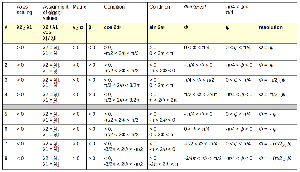
This table tells you exactly what to do if you have a matrix A_q and choose an initial scaling of the half-axes such that

In case 1, you should assign λ_I (see eq. (101)) to λ₁ and λ_II (see eq. (102)) to λ₂ , in case 2 you should do the opposite. From the λ-values you then get the length of the respective half-axes. The rotation angle then follows from ψ as it was defined in eq. (50). This prescription can directly be encoded in Python programs.

Testing another helper angle : We could also have used another helper angle as e.g.

Then ω flips signs with β and (λ₂ – λ₁). The following table shows the effect:

Table 2 – rotation angle determination for different cases and helper angle ω

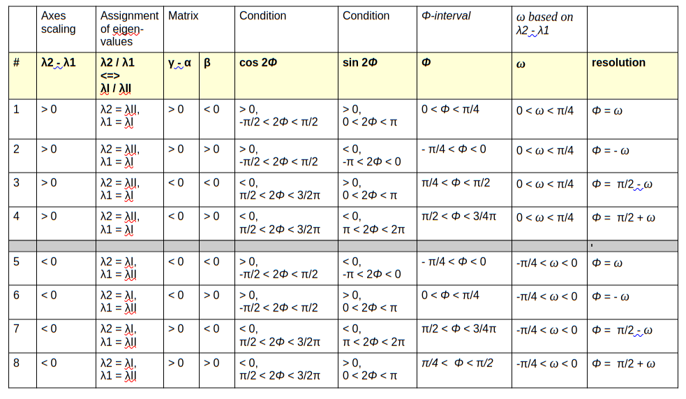
You see that as long as (λ₂ – λ₁) and (γ – α) have the same sign, then only the sign of β is relevant for the calculation of Φ.

Simplification for the determination of the rotation angle

Now, we come to an important point: If you look just from a geometrical point of view onto the tables and take into account the symmetries of an ellipse, you see that for given (fixed) values of α, β and γ

• case #7 in the table is equivalent to case #1,
• case #8 is equivalent to case#2,
• case#5 is equivalent to case #3
• and case #6 is equivalent to case #4.

I leave it to the reader to visualize this with some schematic drawings. Please, also mark the upper part of both axes whilst rotating. You will see that we get an exact match of the final ellipse. I will provide plots for real examples in one of the next posts.

Actually, the equivalence of the named cases is a a natural thing: We can get one and the same target ellipse from two initial configurations of an axis-parallel ellipse: Either the longer or the shorter axis is aligned with the x-axis. The angle to one and the same rotated ellipse is different by just π/2.

Our result means two things:

1. The upper part of the table covers already all visually identical cases.
2. The ambiguity in discriminating between Case 1 and Case 2 can be resolved:
3. When we get a matrix A_q describing some elliptic data, we can always choose (λ₂ – λ₁) > 0 and then determine the angle Φ from the upper part of table 1, without missing any solution.

We should see this in numerical tests.

Conclusion

In this post we have derived essential properties of centered, rotated ellipses from two matrix-based representations. Such calculations become relevant when e.g. experimental or numerical data only deliver the coefficients of a quadratic form for the ellipse. We have shown how the elements of relevant matrices are related to quantities like the lengths of the principal axes of the ellipse and the inclination of these axes against the x-axis of the chosen coordinate system.

We have seen that the determination of the ellipse’s rotation angle deserves some precision. Determining the right angle depends on characteristic properties of the matrix elements. We have to follow some rules which I have given in a table.

In one of the next posts of this mini-series,

Ellipses via matrix elements – II – numerical tests of formulas

I will briefly show plots of numerical examples, which illustrate some of the results of the present post.