Properties of BVD confidence ellipses – I – constant limits and tangents in x- and y-direction during variation of the Pearson correlation coefficient

We have gathered a lot of knowledge about Bivariate Normal Distributions [BVDs] and their contour ellipses in the math section of this blog. We can now analyze some secondary and funny properties of BVD contour and confidence ellipses. Among other things the variation of some key properties with the Pearson correlation coefficient ρ is of interest for data analysts.

In this post I am looking at special points on a BVD based confidence ellipse, namely points which have either an extreme x– or an extreme y-coordinate. At these points we find vertical and horizontal tangents of the ellipse. We compute the dependence of the coordinates of respective points on the correlation coefficient ρ and determine the positions of the axis-parallel tangents to confidence ellipses. We will find that the tangents’ positions do not change when we vary the correlation coefficient, only, and keep other BVD and ellipse parameters constant. The ellipses get boxed by a rectangle whose dimensions depend on a given Mahalanobis distance and the standard deviations of the BVD’s marginals.

Knowledge about BVDs and ellipses may be required to fully understand the contents of this post. The posts [1] to [8] which I have listed in the last section provide respective information and mathematical derivations.

Relevant matrices – covariance matrix and its inverse

We use the elements of the usual matrices, which control the probability density function [pdf] of a BVD, namely the covariance matrix Σ and its inverse Σ^-1 . See [1] for more details and formulas.

\[ \begin{align} &\pmb{\Sigma} \,=\, \begin{pmatrix} \sigma_x^2 &\rho\, \sigma_x\sigma_y \\ \rho\, \sigma_x\sigma_y & \sigma_y^2 \end{pmatrix} \,, \tag{1} \\[10pt] &\pmb{\Sigma}^{-1} \,=\, {1 \over \sigma_x^2\, \sigma_y^2\, \left( 1\,-\, \rho^2\right) } \, \begin{pmatrix} \sigma_y^2 &-\rho\, \sigma_x\sigma_y \\ -\rho\, \sigma_x\sigma_y & \sigma_x^2 \end{pmatrix} \\[10pt] &\quad \quad =\, \begin{pmatrix} \alpha & \beta/2 \\ \beta/2 & \gamma \end{pmatrix} \,, \tag{2} \\[10pt] & \pmb{\Sigma} \bullet \pmb{\Sigma}^{-1} \,=\, \mathbf I_n \,. \tag{3} \end{align} \]

σ_x and σ_y are the standard deviations of the BVD’s marginal distributions along the x– and y-axes. ρ is the Pearson correlation coefficient.

For a regular BVD these matrices have to be symmetric, invertible and positive-definite. They define BVDs which can be centered in a Cartesian coordinate system [CCS]. Respective centered contour ellipses for a constant probability density are given by quadratic forms mediated by matrix Σ^-1; see [2] for matrix-defined ellipses. The Mahalanobis distance d_m defines a BVD ellipse’s diameters via an equation for vectors v_E reaching from the origin to points on the (centered) ellipse:

\[ \begin{align} \left(d_m\right)^2 \,:=\, {\pmb{v}}^T_E \bullet \, \pmb{\Sigma}^{-1} \bullet {\pmb{v}}_E \,. \tag{4} \end{align} \]

The Mahalanobis distance corresponds to a certain level of constant probability density. It is related to a confidence level P via the following equation:

\[ d_m \:=\: d_m\left(P\right) \:=\: \sqrt{ \,-\, 2 \, \ln \left(\, 1 \,-\, P\, \right) } \,. \tag{5}\]

See [3] and [4] for more details.

Examples and plots

The following picture shows the variation of contour ellipses of BVDs with constant standard deviations for a Mahalanobis distance d_m = 1 and a respective confidence level of P = 0.393. The BVDs, for which I have plotted the confidence ellipses, have the following characteristic data – with only the Pearson correlation coefficient ρ being varied:

σ_x= 1.4, σ_y = 2.5, 0 ≤ ρ < 1.
ρ = 0.1, 0.2, 0.4, 0.6, 0.8, 0.9, 0.99, 0.9999.

Regarding the rotation angle of the ellipses all ellipses reflect “case 3” distinguished in [2]. The image data have been computed with the help of an eigendecomposition of Σ^-1 (see [2]). The ellipses numbered from 0 to 7 reflect the growing ρ-values given above – in this order.

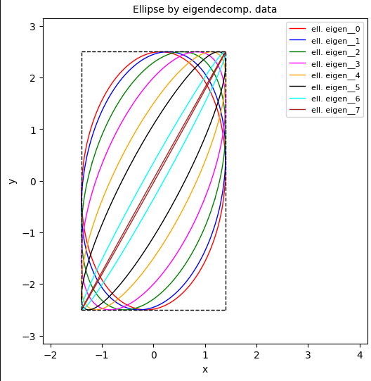
BVD contour ellipses with varying Pearson coefficient

We clearly see the effect of the varying correlation coefficient ρ. When we keep the standard deviations σ_x and σ_y of the BVD’s marginals (along the CCS-axes) constant, all the ellipses appear to be boxed in a rectangle. Looking at the coordinate values of the corner-points we get the idea that the corners of this rectangle are actually defined by ± σ_x and ± σ_y.

Furthermore, at points with either extremal x– or y-coordinates the sides of the rectangle seem to touch the ellipses tangentially. The line which the narrowing ellipses approach with ρ→1 appears to be defined by the diagonal of the rectangle. (And not by an angle Φ = π/4 as you may have learned for standardized normal distributions). If our assumptions were really true, this would also give us a condition on the longer half-axis h_L for ρ→1:

\[ \begin{align} \sigma_y \gt \sigma_x \, \land \, \rho \, \rightarrow \, 1 \,\land \, d_m\,=\, 1\, \,: \quad \tan(\phi) \,& =\, \sigma_y / \sigma_x \,, \tag{6} \\[10pt] h_{L} \,&=\, \sqrt{ \, \sigma_x^ 2 \,+\, \sigma_y^ 2 \, } \,. \tag{7} \end{align} \]

The next plot shows data for a varying negative correlation coefficient ρ:

σ_x= 2.1, σ_y = 0.8, -1 < ρ ≤ 0.
ρ = -0.1, -0.2, -0.4, -0.6, -0.8, -0.9, -0.99, -0.9999.

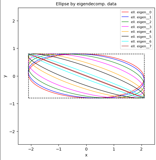
BVD contour ellipses with varying negative Pearson coefficient

This situation corresponds to “case 2” distinguished in [2]. We again see a limiting rectangular box with side coordinates close to ± σ_x and ± σ_y. So, in the depicted situation, we have

\[ \begin{align} \sigma_y \lt \sigma_x \, \land \, \rho \, \rightarrow \, -1 \, \,\land \, d_m\,=\, 1 \,\,: \quad \tan(\phi) \,& =\, – \, \sigma_y / \sigma_x \,, \tag{8} \\[10pt] h_{L} \,&=\, \sqrt{ \, \sigma_x^ 2 \,+\, \sigma_y^ 2 \, } \,. \tag{9} \end{align} \]

Can we mathematically prove the indicated properties of BVD confidence ellipses for a variation of the correlation of a BVD’s marginals? And can we generalize them somehow for d_m ≠ 1 ? Yes, with the mathematical equipment gathered already, we can …

Proof A for the extreme coordinates of points limiting a confidence ellipses in x– and y-direction

Our suspicion is that the extremal coordinate values, which certain points on our ellipses can assume, are given by –σ_x, +σ_x, in x-direction and –σ_y, +σ_y in y-direction. The respective other coordinates of the extremal points and their dependence on ρ must still be analyzed.

We start our mathematical considerations with the fact that Σ^-1 defines a quadratic form for an ellipse. We observe eq. (2) and get the following condition for d_m= 1:

\[ \alpha * x^ 2 \,+\, \beta * x\,y \,+\, \gamma*y^ 2 \,=\, 1 \,. \tag{10}\]

Note that this equation is totally symmetric regarding the roles of x and y! We will use this property later on. Note also that any different Mahalanobis distance d_m ≠ 1 (see [4]) could be accounted for by replacing the sigma-values σ_x and σ_y in the definition of α, β and γ by (σ_x * d_m) and (σ_y*d_m).

Note further that for a BVD we require that the following inequalities are fulfilled to guarantee the invertibility and positive definiteness of matrix Σ^-1:

\[\alpha \gt 0, \,\, \gamma \gt 0 \,\, \land \, {\text{det}} \left( \operatorname{\pmb{\Sigma^{-1}}} \right) \:=\: \alpha*\gamma \,-\, {1 \over 4}\, \beta^2 \:\gt\: 0 \,. \tag{11} \]

By using a quadratic completion we can rewrite eq. (10) as

\[ \left[ y \,+\, {1\over2}\, {\beta \over \gamma} * x \right]^2 \,=\, {1\over \gamma} \,-\, \left( \, {\alpha \over \gamma} \,-\, {1\over 4}\, \, {\beta^2 \over \gamma^2} \, \right) * x^2 \,\, (\ge 0) \,. \tag{12} \]

This gives us the solutions y(x)

\[ y \,=\, – \, {1\over 2} \,{\beta \over \gamma} *x \,\pm \, \left[\, {1\over \gamma} \,-\, \left( \, {\alpha \over \gamma} \,-\, {1\over 4}\, \, {\beta^2 \over \gamma^2} \, \right) * x^2 \,\right]^{1/2} \,. \tag{13} \]

While α, γ > 0, β can switch its sign, dependent on ρ. We know the orientation of the ellipses for different signs of ρ already very well; see e.g. [7]. Therefore, extremal values are achieved for

\[ \rho \,\ge\, 0 \,\land\, x \,\gt\, 0 \,\,: \quad y_{max} \,=\, – \, {1\over 2} \,{\beta \over \gamma} *x \,+\, \left[\, {1\over \gamma} \,-\, \left( \, {\alpha \over \gamma} \,-\, {1\over 4}\, \, {\beta^2 \over \gamma^2} \, \right) * x^2 \,\right]^{1/2} \,, \tag{14} \]

\[ \rho \,\gt\, 0 \,\land\, x \,\lt\, 0 \,\,: \quad y_{max} \,=\, – \, {1\over 2} \,{\beta \over \gamma} *x \,-\, \left[\, {1\over \gamma} \,-\, \left( \, {\alpha \over \gamma} \,-\, {1\over 4}\, \, {\beta^2 \over \gamma^2} \, \right) * x^2 \,\right]^{1/2} \,. \tag{15} \]

Similar relations hold for other conditions. We keep this in mind.

Extremal y-values

Our central condition for an extremal value of y(x) is:

\[ {\partial \,y(x) \over \partial \, x} \,=\, 0 \,.\tag{16} \]

This means

\[ -\, {1\over 2}\, {\beta \over \gamma} \,\mp \, { \left(\, {\alpha / \gamma} \,-\, {1/4}\, \, ({\beta^2 / \gamma^2}) \, \right) *x \over \left[ \, {1/ \gamma} \,-\, \left( \, {\alpha / \gamma} \,-\, {1/ 4}\, \, ( {\beta^2 /\gamma^2}) \, \right) * x^2 \,\ \right]^{1/2} } \,=\, 0 \,. \tag{17} \]

Squaring gives

\[{1\over4} \, {\beta^2 \over \gamma^2} \, \left[ \, {1 \over \gamma} \,-\, \left( \, {\alpha \over \gamma} \,-\, {1 \over 4}\, \, ( {\beta^2 \over \gamma^2}) \, \right) * x^2 \,\ \right] \,=\, \left[ \, {\alpha \over \gamma} \,-\, {1 \over 4}\, \, ( {\beta^2 \over \gamma^2}) \, \right]^2 * x^2 \,. \tag{18} \]

We solve the equation for x and get

\[ x \,=\, \pm \, {\beta \over \gamma } \,\left[ \, \alpha \, \left( \, {\alpha \over \gamma} \,-\, {1 \over 4}\, \, ( {\beta^2 \over \gamma^2}) \, \right) \right]^{-1/2} \tag{19} \]

Filling in the standard deviations and the correlation coefficient for the elements of Σ^-1 according to eq. (2) leads to

\[ x \,=\, \pm \ \rho * \sigma_x \,. \tag{20} \]

Inserting these results in into (10) and (11) and observing respective rules for the extreme values gives us

\[ \begin{align} y_{max} \,&=\, + \, \sigma_y \,, \,\, \text{for } \ x \,\ge\, 0 \,\land\, \rho \gt 0 \,, \\[10pt] y_{max} \,&=\, – \, \sigma_y \,, \,\, \text{for } \ x \,\lt\, 0 \,\land\, \rho \gt 0 \,, \\[10pt] y_{max} \,&=\, + \, \sigma_y \,, \,\, \text{for } \ x \,\le\, 0 \,\land\, \rho \lt 0 \,, \\[10pt] y_{max} \,&=\, – \, \sigma_y \,, \,\, \text{for } \ x \,\gt\, 0 \,\land\, \rho \lt 0 \,. \end{align} \tag {21} \]

Mahalanobis distances d_m ≠ 1

You may now ask yourself how the proof would have worked for contour ellipses corresponding to another value of the Mahalanobis distance d_m. Nothing much would have changed. You just replace the sigma-values σ_x and σ_y by (σ_x * d_m) and (σ_y* d_m), and arrive at or final result

\[ x \,=\, \pm \, \rho * d_m * \sigma_x \,. \tag{22} \]

\[ \begin{align} y_{max} \,&=\, + \, d_m * \sigma_y \,, \,\, \text{for } \ x \,\ge\, 0 \,\land\, \rho \gt 0 \,, \\[10pt] y_{max} \,&=\, – \, d_m * \sigma_y \,, \,\, \text{for } \ x \,\lt\, 0 \,\land\, \rho \gt 0 \,, \\[10pt] y_{max} \,&=\, + \, d_m * \sigma_y \,, \,\, \text{for } \ x \,\le\, 0 \,\land\, \rho \lt 0 \,, \\[10pt] y_{max} \,&=\, – \, d_m * \sigma_y \,, \,\, \text{for } \ x \,\gt\, 0 \,\land\, \rho \lt 0 \,. \end{align} \tag {23} \]

Extremal x-values

As said: Eq. (10) is fully symmetric regarding the roles of x and y. We, therefore, can directly conclude for the y– and x-coordinates coordinates of points on our ellipse with extremal x-values:

\[ y \,=\, \pm \, \rho * d_m * \sigma_y \,. \tag{24} \]

\[ \begin{align} x_{max} \,&=\, + \, d_m * \sigma_x \,, \,\, \text{for } \ x \,\ge\, 0 \,\land\, \rho \gt 0 \,, \\[10pt] x_{max} \,&=\, – \, d_m * \sigma_x \,, \,\, \text{for } \ x \,\lt\, 0 \,\land\, \rho \gt 0 \,, \\[10pt] x_{max} \,&=\, + \, d_m * \sigma_x \,, \,\, \text{for } \ x \,\le\, 0 \,\land\, \rho \lt 0 \,, \\[10pt] x_{max} \,&=\, – \, d_m * \sigma_x \,, \,\, \text{for } \ x \,\gt\, 0 \,\land\, \rho \lt 0 \,. \end{align} \tag {25} \]

The rotation angle of a (centered) confidence ellipse for maximal correlation

Let us show that the angle Φ by which the contour ellipse (more precisely its longer half-axis) is rotated against the CCS is indeed given by eqs. (6) and (8) for the case d_m = 1. Going through post [2] we find some key conditions regarding the rotation angle of a respective ellipse:

\[ \begin{align} \gamma \,-\, \alpha \,&=\, ( \lambda_2 \,-\, \lambda_1) \, \cos(2\phi) \,, \tag{26} \\[10pt] -\, \beta \,&=\, ( \lambda_2 \,-\, \lambda_1) \, \sin(2\phi) \,, \tag{27} \end{align} \]

with the lambda-values being related to the half-axes. This gives us

\[ \tan\left(2 \, \phi\right) \,=\, { -\, \beta \over \gamma \,-\, \alpha } \,. \tag{28}\]

Using eq. (2) for the elements of Σ^-1 (and d_m = 1) leads to

\[ \tan\left(2 \, \phi\right) \,=\, \rho * 2 \, {\sigma_y \over \sigma_x} \, \left[ \, 1 \,-\, \left({\sigma_y \over \sigma_x}\right)^2 \, \right]^{-1} \,. \tag{29} \]

Now, we set

\[\rho \,= \, \pm\, 1 \tag{30} \]

and remember an elementary trigonometric relation, namely

\[ \tan\left(2\,\phi\right) \,=\, 2\, \tan(\phi) \,\left[\, 1 \,-\, \tan^2(\phi) \, \right]^{-1} \,. \tag{31} \]

A comparison with eq. (29) and use of (30) gives us the aspired result for d_m = 1

\[\begin{align} \rho \,=\, +1 \,\,&: \quad \tan(\phi) \,= \, +\, {\sigma_y \over \sigma_x} \,, \tag{32} \\[10pt] \rho \,=\, -1 \,\,&: \quad \tan(\phi) \,= \, -\, {\sigma_y \over \sigma_x} \,. \tag{33} \end{align} \]

This confirms eqs. (7) and (9) for the longer half-axis h_L (for d_m = 1):

\[ \rho \,=\, \pm\, 1 \,\, : \quad h_L \,=\, \sqrt{ \, \sigma_x^ 2 \,+\, \sigma_y^ 2 \, } \,. \tag{34} \]

For d_m ≠ 1 we need to stretch the concentric ellipses and apply the respective sigma-replacements. We get

\[ \rho \,=\, \pm\, 1 \,\, : \quad h_L \,=\, d_m * \sqrt{ \, \sigma_x^ 2 \,+\, \sigma_y^ 2 \, } \,. \tag{35} \]

Boxed ellipses

Taking all of our above results into account, we really can speak of “boxed confidence ellipses“. The ellipses’ extensions in x,y-directions are limited by a centered and axis-parallel rectangle, whose corner-points are given by

(- d_m*σ_x, – d_m*σ_y ), (+ d_m*σ_x, – d_m*σ_y ), (+ d_m*σ_x, + d_m*σ_y ), (- d_m*σ_x, + d_m*σ_y ).

The rectangle’s sides touch the ellipses tangentially. For maximum correlation the smaller half-axes of the ellipses approaches zero and the longer diameter coincides with the diagonal of the rectangle.

Proof B for extremal coordinate values of the ellipses

Just to show you that other methods to define a contour or confidence ellipse of a BVD are consistent, we use another definition of a contour ellipse, namely its parameterization (see [5]) by an angle and the Mahalanobis distance d_m:

\[ \begin{align} x \:&=\: \sigma_x * d_m * \cos \phi \,, \tag{36} \\[10pt] y\:&=\: \sigma_y * d_m * \left( \, \rho * \cos \phi \,+\, \sqrt{\, 1 \,-\, \rho^2 \, } * \sin \phi \, \right) \,, \tag{37} \\[10pt] 0 &\le \phi \,\le\, 2\,\pi \,, \quad d_m \:=\: const. \, . \tag{38} \end{align} \]

We can replace d_m * cos(Φ) by x/σ_x to get:

\[ y \:=\: \sigma_y \, \left[\, \rho * {x \over \sigma_x} \,\pm\, d_m * \sqrt{\, 1 \,-\, \rho^2 \, } * \sqrt{\, 1 \,-\, x^2 /(d_m^2 \, \sigma_x^2) \,} \, \right] \,. \tag{39} \]

Here again similar conditions as considered ahead of eqs. (11) and (12) apply for the extremal values for different signs of ρ. I only look at extremal y-values. We combine the condition (16) for extrema with (39) to get

\[ {\sigma_y \over \sigma_x} \, \rho \, \sqrt{\, 1 \,-\, x^2 /(d_m^2 \, \sigma_x^2) \,} \,=\, \mp\, { \sigma_y \over d_m \, \sigma_x^2 } \, \sqrt{\, 1 \,-\, \rho^2 \, } * x \,. \tag{40}\]

Squaring, reordering and solving for x again results in

\[ \begin{align} x \,=\, \pm \, \rho * d_m * \sigma_x \,, \tag{41} \\[10pt] y_{max} \,=\, \pm \, d_m * \sigma_y\,. \tag{42} \end{align}\]

Of course, we once again had to evaluate the different situations for negative and positive values of ρ.

The derivation of y, x_max coordinate values for extremal points in x-direction requires the application of some trigonometric relations to eqs. (36) and (37) first, but moves along a very similar path as for y_max afterward. I leave the respective proof to the reader.

Conclusion

In this post we have seen how contour or confidence ellipses of a BVD vary with the Pearson correlation coefficient ρ. We saw that they are confined by an axis-parallel rectangle. The corner points of the rectangle are given by coordinates equal to the Mahalanobis distance times positive/negative values of the standard deviations of the BVD’s marginals in x– and y-direction. The rectangle’s sides touch the ellipses tangentially. For maximum correlation the longer diameter of the ellipse approaches the diagonal of the rectangle, whilst the other diameter approaches zero. .

In the next post on properties of a BVDs contour and confidence ellipses we prove the behavior of the diameters with varying correlation independently.

Links and references

[1] R. Mönchmeyer, 2025, “Bivariate normal distribution – derivation by linear transformation of a random vector of two independent Gaussians”,
https://machine-learning.anracom.com/2025/06/24/bivariate-normal-distribution-derivation-by-linear-transformation-of-random-vector-of-two-independent-gaussians/

[2] R. Mönchmeyer, 2025, “Ellipses via matrix elements – I – basic derivations and formulas”,
https://machine-learning.anracom.com/2025/07/17/ellipses-via-matrix-elements-i-basic-derivations-and-formulas

[3] R. Mönchmeyer, 2025, “Bivariate Normal Distribution – Mahalanobis distance and contour ellipses”,
https://machine-learning.anracom.com/2025/07/03/bivariate-normal-distribution-mahalanobis-distance-and-contour-ellipses/

[4] R. Mönchmeyer, 2025, “Bivariate Normal Distribution – integrated probability up to a given Mahalanobis distance, the Chi-squared distribution and confidence ellipses”,
https://machine-learning.anracom.com/2025/07/30/bivariate-normal-distribution-integrated-probability-up-to-a-given-mahalanobis-distance-the-chi-squared-distribution-and-confidence-ellipses

[5] R. Mönchmeyer, 2025, “BivariateNormal Distributions – parameterization of contour ellipses in terms of the Mahalanobis distance and an angle”,
https://machine-learning.anracom.com/2025/07/07/bivariate-normal-distributions-parameterization-of-contour-ellipses-in-terms-of-the-mahalanobis-distance-and-an-angle/

[6] R. Mönchmeyer, 2025, “Cholesky decomposition of an ellipse-defining symmetric matrix”,
https://machine-learning.anracom.com/2025/07/20/cholesky-decomposition-of-an-ellipse-defining-symmetric-matrix/

[7] R. Mönchmeyer, 2025, “Ellipses via matrix elements – II – numerical tests of formulas”,
https://machine-learning.anracom.com/2025/07/23/ellipses-via-matrix-elements-ii-numerical-tests-of-formulas/

[8] R. Mönchmeyer, 2024, “Bivariate Normal Distribution – derivation of the covariance and correlation by integration of the probability density”,
https://machine-learning.anracom.com/2024/07/09/bivariate-normal-distribution-derivation-of-the-covariance-and-correlation-by-integration-of-the-probability-density/

[9] R. Mönchmeyer, 2024, “Probability density function of a Bivariate Normal Distribution – derived from assumptions on marginal distributions and functional factorization”,
https://machine-learning.anracom.com/2024/07/07/probability-density-function-of-a-bivariate-normal-distribution-derived-from-assumptions-on-marginal-distributions-and-functional-factorization/