Multivariate Normal Distributions – III – Variance-Covariance Matrix and a distance measure for vectors of non-degenerate distributions

In previous posts of this series I have motivated the functional form of the probability density of a so called “non-degenerate Multivariate Normal Distribution“.

Multivariate Normal Distributions – II – Linear transformation of a random vector with independent standardized normal components
Multivariate Normal Distributions – I – Basics and a random vector of independent Gaussians

In this post we will have a closer look at the matrix Σ that controls the probability density function [pdf] of such a distribution. We will show that it actually is the covariance matrix of the vector distribution. Due to its properties the inverse of Σ can be used to define a special measure for the distance of the distribution’s vectors from their mean vector. Setting this distance to a constant value defines a contour surface of the probability density and gives rise to quadratic forms describing surfaces of multidimensional ellipsoids.

While we dive deeper into mathematical properties we should not forget that our efforts have the goal to analyze real vector distributions appearing in Machine Learning processes. Numerically evaluated hyper-contours which are close to multidimensional ellipsoids would be one of multiple indicators of an underlying multidimensional normal distribution. We will also dare a first look into the topic of degenerate normal distributions.

We abbreviate the expression “Multivariate Normal Distribution” by either MND or, synonymously MVN. Both abbreviations appear in the literature. We refer to the “variance-covariance matrix” of a random vector just as its “covariance matrix”.

Probability density function and normalization

Our idea of a random vector Y_N giving a non-degenerate MND is based on the application of an invertible linear transformation onto a random vector Z representing a continuous distribution of vectors z whose component values follow independent and standardized 1-dimensional normal distributions :

\[ \pmb{Z} = \left(Z_1, \, Z_2, \, ….., \,Z_n \right)^T \,\sim\, \pmb{\mathcal{N}}_n \left(\pmb{0},\, \pmb{\operatorname{I}} \right) \]

\[ \pmb{Y}_N \,=\, \left(Y_1, \, Y_2, \, ….., \, Y_n \right)^T \: = \: \pmb{\operatorname{M}}_{\small Y} \, {\small \bullet} \, \pmb{Z} + \pmb{\mu}_y \, , \quad \pmb{Y}_N \,\sim\, \pmb{\mathcal{N}}_n \left(\pmb{\mu}_{\small Y},\, \pmb{\Sigma}_{\small Y} \right) \]

For details of Z see post I. M_y is some (n x n)-matrix representing the transformation. Remember that the z-vector distribution had a pdf

\[ g_{Z}(\pmb{z}) \, =\, {1 \over \sqrt{(2\pi)^n} } \, {\large e}^{ – \, {\Large 1 \over \Large 2} \left( {\Large \pmb{z}^T \, \bullet \, \pmb{z}} \right) } \, , \]

with contour hyper-surfaces being n-dimensional spheres. An evaluation of the transformation gave us a pdf g_y(y) for the distribution of the transformed vectors y = M_yz ( with y, z ∈ ℝⁿ) :

\[ g_{\small Y}(\pmb{y}) \,=\, {1 \over (2\pi)^{n/2} \, \left(\operatorname{det}\pmb{\operatorname{\Sigma}}_{\small Y}\right)^{1/2} } \, {\large e}^{ – \, {\Large 1 \over \Large 2} \, \left[ \left( {\Large \pmb{y} \,-\, \pmb{\mu}_y } \right)^{\Large T} \, { \Large \pmb{\operatorname{\Sigma}}_{\small Y}^{-1} } \, \left( {\Large \pmb{y} \,-\, \pmb{\mu}_y } \right) \right] } \, . \]

Σ_Y is a symmetric and invertible matrix defined by

\[ \pmb{\operatorname{\Sigma}}_{\small Y} \, = \, \pmb{\operatorname{M}}_{\small Y}\, \pmb{\operatorname{M}}_{\small Y}^T \, . \]

The factor in front is just a normalization factor (coming, of course, from Z). By our MND-construction we actually have found the useful formula :

\[ \begin{align} 1 \, &= \, {1 \over \sqrt{(2\pi)^n} } \, \int_{-\infty}^{\infty}\int_{-\infty}^{\infty} \cdots \int_{-\infty}^{\infty} {\large e}^{ – \, {\Large 1 \over \Large 2} {\Large \boldsymbol{z}\boldsymbol{z}^T} }dz_1dz_2 \cdots dz_n \\ &= \, {1 \over (2\pi)^{n/2} \, \left|\pmb{\operatorname{\Sigma}}_{\small Y}\right|^{1/2} } \, \int_{-\infty}^{\infty}\int_{-\infty}^{\infty} \cdots \int_{-\infty}^{\infty} {\large e}^{ – \, {\Large 1 \over \Large 2} \, \left[ \left( {\Large \pmb{y} \,-\, \pmb{\mu}_{\small Y} } \right)^T \, { \Large \pmb{\operatorname{\Sigma}}_{\small Y}^{-1} } \, \left( {\Large \pmb{y} \,-\, \pmb{\mu}_{\small Y} } \right) \right] } dy_1dy_2 \cdots dy_n \end{align} \]

You can prove this by using the Jacobi determinant of the transformation. In the sense of post I Y_N is mapping objects onto a continuous distribution of vectors y ∈ ℝⁿ being connected to vectors z given by another random vector Z. Note that we describe the vectors and their components in an Euclidean Coordinate System [ECS] spanning the ℝⁿ .

Getting the “variance-covariance matrix” from the probability density

In post I of this series we defined the “variance-covariance matrix” of a random vector and the related vector distribution. An application gives us :

\[ \begin{align} \operatorname{Cov}\left(\pmb{Y}_N\right) \: &:= \: \operatorname{\mathbb{E}}\left[ \left(\pmb{Y_N} – \pmb{\mu}_{\small Y} \right) \, \left(\pmb{Y_N} – \pmb{\mu}_{\small Y} \right)^T \right] \\ &= \: \operatorname{\mathbb{E}}\left[ \left(\pmb{\operatorname{M}}_{\small Y} \pmb{\operatorname{Z}} \right) \, \left(\pmb{\operatorname{M}}_{\small Y} \pmb{\operatorname{Z}} \right)^T \right] \\ &= \: \pmb{\operatorname{M}}_{\small Y} \operatorname{\mathbb{E}}\left[ \pmb{Z} \pmb{Z}^T \right] \pmb{\operatorname{M}}_{\small Y}^T \\ &= \: \pmb{\operatorname{M}}_{\small Y} \, \pmb{\operatorname{I}} \, \pmb{\operatorname{M}}_{\small Y}^T \,=\, \pmb{\operatorname{\Sigma}}_{\small Y} \, ! \end{align} \]

So, actually our symmetric Matrix Σ_Y = M_y • M_y^T is nothing else than the variance-covariance matrix of our random vector Y_N .

Note that symmetry does in no way imply a diagonality of the matrix. On the contrary: For a general M_y the resulting off-diagonal elements of Σ_Y will assume non-zero values. In contrast to the previously discussed normal distributions W and Z with independent components, this indicates that we will in general find a correlation between the components of the transformed random vector Y_N. We will later see that this has a geometrical interpretation

Positive-definite covariance matrix?

A symmetric matrix is invertible if it is positive-definite. Can we find out about this? By definition for a real valued matrix like Σ_Y we request for any vector y ∈ ℝⁿ other then the zero vector 0 :

\[ \pmb{y}^T \, \pmb{\operatorname{\Sigma}}_{\small Y} \, \pmb{y} \, \gt \, 0 \]

Replacing Σ_Y by the automorphism M_y and M_y^T we get:

\[ \begin{align} \pmb{y}^T \, \pmb{\operatorname{\Sigma}}_{\small Y} \, \pmb{y} \,&=\, \pmb{y}^T \pmb{\operatorname{M}}_{\small Y} \pmb{\operatorname{M}}_{\small Y}^T \pmb{y} \\ \,&=\, \left( \pmb{\operatorname{M}}_{\small Y}^T \pmb{y} \right)^T \, \left( \pmb{\operatorname{M}}_{\small Y}^T \pmb{y} \right) \\ \,&=\, \sum\limits_{j=1}^n q_j^2 \geq 0\,,\:\, \mbox{with} \,\: \pmb{q} = \pmb{\operatorname{M}}_{\small Y}^T \, \pmb{y}\, . \end{align} \]

For a real valued invertible (n x n)-matrix M_y^T the equal sign comes about only for the trivial case y = 0. So, we have a positive definite matrix. Note that we could have also derived this from back-transforming y to a z vector by using the inverse of M_y and by evaluation of the matrix products to become the identity matrix.

Actually, Linear Algebra teaches us that any real-valued symmetric matrix A is positive definite if there exists a real non-singular matrix M such that A = M • M^T ( see e.g. [1]). And: A positive semi-definite and invertible matrix is positive-definite! So, we could have directly concluded it from our definitions. But note that the derivation above holds also for more general cases of M.

Consistency check, just for completeness: If M is invertible, so is M^T and, therefore, M^T • x = 0 only has the trivial solution x = 0. Thus: With an invertible M, the matrix Σ = MM^T becomes symmetric (by construction!) and positive-definite – and thus invertible! In addition this is consistent with the fact that a quadratic M with full rank (n!) is invertible. But if M has full rank, then M^T has, too, and also the matrix product MM^T! The latter follows from

\[ \begin{align} &\operatorname{rank}\left(\pmb{\operatorname{A}}*\pmb{\operatorname{B}}\right) \,\le \,\operatorname{min}\left(\operatorname{rank}\left(\pmb{\operatorname{A}}\right), \,\operatorname{rank}\left(\pmb{\operatorname{B}}\right)\right) \\ &\operatorname{rank}\left( \pmb{\operatorname{A}}*\pmb{\operatorname{B}}\right) \,\ge\, \operatorname{rank}\left( \pmb{\operatorname{A}}\right) \,+\, \operatorname{rank}\left( \pmb{\operatorname{B}}\right) \,-\, n \\ &\mbox{(Sylvester rank inequality for a (m x n)-matrix} \, \pmb{\operatorname{A}} \, \\ &\mbox{and a (n x k)-matrix} \, \pmb{\operatorname{B}} \end{align} \]

and setting B = A^T. See e.g. [2] .

The transpose and the inverse of the covariance matrix Σ_Y are positive definite, too

It is relatively easy to show that the inverse of a positive-definite matrix A is positive-definite, too. First we can show that A^T is positive definite. Because the matrix product (x^T A x) is a scalar we have:

\[ \pmb{x}^T \pmb{\operatorname{A}} \pmb{x} \, = \, \left( \pmb{x}^T \pmb{\operatorname{A}} \pmb{x} \right)^T \,=\, \pmb{x}^T \pmb{\operatorname{A}}^T \pmb{x} \gt 0, \,\, for \, \, \pmb{x} \ne \pmb{0} \]

and we get positive values as for A itself. Now, let us take a vector y = Ax. Then

\[ \pmb{y}^T \pmb{\operatorname{A}}^{-1} \pmb{y} = \pmb{x}^T \pmb{\operatorname{A}}^T \pmb{\operatorname{A}}^{-1} \pmb{\operatorname{A}} \pmb{x} \,= \, \pmb{x}^T \pmb{\operatorname{A}}^T \pmb{x} \gt 0\,, \,\, for \, \, \pmb{x} \ne \pmb{0} \]

So, we know for our special case of non-degenerate normal distributions that Σ_Y^-1 is both symmetric and positive-definite.

The “Mahalanobis distance” d_N of a non-degenerate multivariate normal vector distribution

For a 1-dimensional Gaussian distribution

\[ g(x, \, \mu_x, \, \sigma_x) \: = \: {1 \over {\sigma * \sqrt{2\pi} } } \, {\large e}^{ – \, {\Large 1 \over \Large 2} \left( {\Large x \, – \, \Large \mu_x \over \Large \sigma_x} \right)^2 } \]

we can interpret the square root of the term in the exponent as a distance d_x of x from the mean value μ_x measured in units of the standard variation σ_x.

\[ d_x \,=\, \sqrt{ {1 \over \sigma_x^2 } \left( x – \mu_x \right)^2 } \,=\, {1 \over \sigma_x} |(x – \mu_x) | \]

What about the exponent

\[ \left( { \pmb{y} \,-\, \pmb{\mu}_{\small Y} } \right)^{T} \, {\small \bullet} \, \pmb{\operatorname{\Sigma}}_{\small Y}^{-1} {\small \bullet} \, \left( \pmb{y} \,-\, \pmb{\mu}_{\small Y} \right) \]

appearing in the probability density function g_y(y) for our continuous vector distribution Y? To be able to define a “distance” in the sense of

\[ d_N\left( \pmb{y}, \pmb{\mu}_{\small Y} \right) \,=\, \sqrt{ \left( { \pmb{y} \,-\, \pmb{\mu}_{\small Y} } \right)^{T} \, {\small \bullet} \, \pmb{\operatorname{\Sigma}}_{\small Y}^{-1} {\small \bullet} \, \left( \pmb{y} \,-\, \pmb{\mu}_{\small Y} \right) } \, =: \, \sqrt{\vphantom{(}D_N} \]

we must obviously require that the expression under the square root is a positive real number, i.e. Σ_Y^-1 must be a positive-definite matrix. For our case of non-degenerate normal distributions Y we know that this is the case. So, the exponent in the probability density function for a non-degenerate MVN gives us really a special measure d (y, μ_y) of the distance of a vector y of a non-degenerate normal distribution Y_N from its average vector μ_y.

This distance is called the “Mahalanobis distance” of a vector bing a member of a non-degenerate MVN.

What does a constant Mahalanobis distance mean?

The probability density of a non-degenerate MVN obviously assumes constant values for constant values of D_N and d_N. A condition

\[ D_N = \left( { \pmb{y} \,-\, \pmb{\mu}_{\small Y} } \right)^{T} \, {\small \bullet} \, \pmb{\operatorname{\Sigma}}_{\small Y}^{-1} {\small \bullet} \, \left( \pmb{y} \,-\, \pmb{\mu}_{\small Y} \right) = C = const. \]

restricts the vectors and couples its components. When we break this expression down to the components y_j we get, due to the symmetry of Σ_Y^-1, a term of the form

\[ D_N \,=\, \sum_{i}^n \sum_{j}^n \xi_{i,j} \, y_i y_j = \sum_{i}^n \xi_{i,i}^2 \, y_i^2 \, , + \, \sum_{i}^n \sum_{j, \, j\ne i}^n 2\, \xi_{i,j} \, y_i y_j \,=\, C \]

with the ξ_i,j being the coefficients of Σ_Y^-1. This is obviously a quadratic form. Such a restrictive form for the components of vectors defines n-dimensional ellipsoids, more precisely the surface of ellipsoids. So, e.g. in 3 dimensions we would get hyper-surfaces of the following form for different growing (integer) values of C:

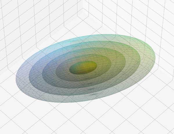
In other forthcoming posts we will see that the axes of these ellipsoids are rotated against the axes of the Euclidean Coordinate System for the ℝⁿ.

Let us look at back to the vectors z of the Z-distribution from which we created our non-degenrate MVN Y_N : All the vectors z fulfilling e.g.

\[ \pmb{z}^T {\small \bullet} \, \pmb{z} \,=\, 1 \]

have a Mahalanobis distance of d_Z = 1 from the origin of our ECS. There endpoints, therefore, reside on the surface of a unit sphere. For some constant value C = z • z^T = const, the z-vectors have endpoints residing on the surfaces of other n-dimensional spheres with different radii. The fact that a linear transformation maps points on a coherent hyper-surface onto points of another coherent hyper-surface indicates that concentric contour-hypersurfaces of our basic Z-distribution are transformed into concentric ellipsoidal contour-hypersurfaces of Y.

We will prove that this is indeed true in the next post. The axes of the ellipsoid are rotated against the axes of the ECS and its midpoint is shifted by μ_y against the ECS origin.

Degeneration and its relation to the transformation “M” and the covariance matrix Σ

The reader may have thought about the word “non-degenerate“. We can understand this a bit better now. The first point is that the probability density function g_y(y) only delivers reasonable values if the determinant of the covariance matrix det(Σ_Y) ≠ 0. For a quadratic symmetric real valued matrix this means invertibility and thus the existence of a Mahalanobis distance measure.

A so called degenerate distribution would be based on a non-quadratic or a non-invertible quadratic matrix M. Σ_Y then would still be symmetric, but not invertible. In these cases a probability function g_y(y) is not defined and does not give us a density in the ℝⁿ. Why?

The reason in case of a singular transformation matrix M is that the transformed distribution Y reduces to some lower dimensional sub-space of ℝⁿ having a dimension m < n. We can conclude this from the fact that the eigenvectors of a non-invertible (symmetric) matrix Σ_Y are not independent of each other. They span a lower dimensional space. This is consistent to the evolution that the density function takes for matrices Σ_Y having determinants closer and closer to zero. In the limit process such a density would become infinitely big as the denominator for g_y(y) indicates.

For non-quadratic matrices the image of the transformation matrix either has a lower dimensionality than the original vectors or the image has a lower dimensionality than the surrounding target space. We will come back in detail to such cases in forthcoming posts.

Thus a singular non-invertible or a non-quadratic transformation M would map a Z–distribution of vectors onto a lower-dimensional sub-space of the ℝⁿ or a surrounding target space ℝ^m (with m > n). While we, for these cases, may not get a reasonably defined density in the target space of the transformation M, the resulting distribution may still have a distance measure and a density defined in a lower dimensional space. We will come back to this point in a later post.

Conclusion

In this post we followed our line of thought for non-degenerate MVNs Y_N which we have defined as the result of invertible linear transformations M applied to a very elementary MND Z ∼ N_n(0, I). Z was based on independent and standardized Gaussian probability densities for the component values of the respective continuously distributed vectors z around a mean vector 0. We found that the matrices Σ and Σ^-1, which define the probability density for Y_N -distributions are symmetric, invertible and – consistently – positive-definite. We could use Σ^-1 to define a distance between vectors of the distribution from its mean vector, the so called Mahalanobis distance. A constant value of this distance defines position vectors whose endpoints reside on the surfaces of multidimensional ellipsoids. We understood that neither the density of a target distribution Y_N created by singular or non-quadratic matrix M would be well-defined.

In the next post of this series

Multivariate Normal Distributions – IV – Spectral decomposition of the covariance matrix and rotation of the coordinate system

we will look at interesting de-compositions (= factorizations) of the covariance matrices of a non-degenerate MVNs and its inverse matrix. This will allow us to understand a non-degenerate MVN as the result of a sequence of special linear transformations.

Links / Literature

[1] “Positive Definite Matrix”, https://mathworld.wolfram.com/ Positive Definite Matrix.html

[2] Wikipedia article on the rank of matrices, https://en.wikipedia.org/ wiki/ Rank_%28 linear_ algebra%29