Midjourney and OpenAI give you access to image generators which create images based on key words in a text prompt. To access Dall-E2 you need to pay money. The tools of Midjourney are no longer free because they have been misused. OpenArt offers you a free service – but the images are public domain. So, some days ago I asked myself whether one can perform prompt based image creation on a Linux PC with a consumer board and a low price graphics card. I should say that my PC is 8 years old …
You maybe assume that something like this is beyond the capabilities of such an old consumer system. Then I stumbled over an interesting article in the Keras-CV documentation: High-performance image generation using Stable Diffusion in KerasCV. This looked very promising and I just had to check it out .
This post below shows that we can indeed run a combination of text transformer and image generator based on the “Stable Diffusion” method with just a few commands. All the credit belongs to the Keras CV team:
Wood, Luke and Tan, Zhenyu and Stenbit, Ian and Bischof, Jonathan and Zhu, Scott and Chollet, Fran\c{c}ois and Sreepathihalli, Divyashree and Sampath, Ramesh and others, KerasCV, 2022. To learn more about KerasCV use this link https://keras.io/keras_cv/.
I have just applied their code to test performance on a Nvidia TI 4060. But the whole stuff is good for some hours of fun …
Requirements
Keras CV requires Keras 3. For TensorFlow users: This in turn requires Tensorflow 2.15 and above. You also have to install the “keras-cv” package (e.g. with pip). While the first sub-version of TF 2.16 gave me some problems in Jupyterlab, the latest builds seem to work well. You may also have to upgrade the “tornado” package to the latest version to avoid some error messages when starting Jupyter Lab. In addition set the NUMA node for your Nvidia card to 0 (see a post in this blog on this topic).
Note that the KerasCV-models require a CUDA capable CPU and GPU for reasonable performance. I have CUDA 12.3 installed on my system. My Python version is 3.11.
Keras CV has done all the work for you … just use the model …
Of course, for text-prompted Stable Diffusion you need pre-trained models. The KerasCV team has done all the work for you. You just need to compile their model. Let me give you the contents of some cells I used. They differ only in details from what the article named above discusses.
Cell1 – reduce warnings
import os
# Suppress some TF2 warnings on negative NUMA node number
os.environ['TF_CPP_MIN_LOG_LEVEL'] = '1'  # or any {'0', '1', '2'}
Cell 2 – Load modules
import time
import keras_cv
#import keras
#import nvidia_smi
import matplotlib.pyplot as plt
import tensorflow as tf   # It loads Keras 3 !
Cell 3 – Prepare your Nvidia card
# Check GPU and activate jit to accelerate
# *************************************************
# NOTE: To change any of the following values you MUST restart the notebook kernel !

b_tf_CPU_only      = False   # we need to work on a GPU
tf_limit_CPU_cores = 4
#tf_limit_GPU_RAM   = 2048
#tf_limit_GPU_RAM   = 7200
tf_limit_GPU_RAM   = 8200

if b_tf_CPU_only:
    tf.config.set_visible_devices([], 'GPU')   # No GPU, only CPU
    #tf.config.set_visible_devices([], 'CPU')  # No CPU - DO NOT USE
    # Restrict number of CPU cores
    tf.config.threading.set_intra_op_parallelism_threads(tf_limit_CPU_cores)
    tf.config.threading.set_inter_op_parallelism_threads(tf_limit_CPU_cores)
else:
    #tf.config.set_visible_devices([], 'CPU')   # No CPU
    gpus = tf.config.experimental.list_physical_devices('GPU')
    tf.config.experimental.set_virtual_device_configuration(gpus[0],
        [tf.config.experimental.VirtualDeviceConfiguration(memory_limit = tf_limit_GPU_RAM)])

# JiT optimizer
tf.config.optimizer.set_jit(True)
# List available CUDA devices
tf.config.experimental.list_physical_devices()
Cell 4 – Two functions
def plot_images(images, fig_size=(14,14)):
    plt.figure(figsize=fig_size)
    for i in range(len(images)):
        ax = plt.subplot(1, len(images), i + 1)
        plt.imshow(images[i])
        plt.axis("off")
def plot_sel_image(images, ind=1, fig_size=(12,12)):
    figure = plt.figure(figsize=fig_size)
    ax = plt.subplot(1, 1, 1)
    plt.imshow(images[ind])
    plt.axis("off")
    return figure
Cell 6 – Load the KerasCV model for Stable Diffusion
keras.mixed_precision.set_global_policy("mixed_float16")
b_with_jit = True
if b_with_jit:
    model = keras_cv.models.StableDiffusion(
        img_width=512, img_height=512, jit_compile=True
    )
else:
    model = keras_cv.models.StableDiffusion(
        img_width=512, img_height=512, jit_compile=False
    )

print("Compute dtype:", model.diffusion_model.compute_dtype)
print("Variable dtype:", model.diffusion_model.variable_dtype)
When you run this cell for the very first time Keras model data will be downloaded in h5-format from huggingface.co. This may take some time.
Note: The data will consume a significant space of more than 3.2 GiB on your hard disk or SSD. In my case the model was saved in a sub-directory of my home folder “~/.keras“.
Running this cell comes with a hint regarding conditions and licenses. I explicitly ask the reader to look at the license conditions and user restrictions defined therein:
Attachment A
Use Restrictions
You agree not to use the Model or Derivatives of the Model:
- In any way that violates any applicable national, federal, state, local or international law or regulation;
- For the purpose of exploiting, harming or attempting to exploit or harm minors in any way;
- To generate or disseminate verifiably false information and/or content with the purpose of harming others;
- To generate or disseminate personal identifiable information that can be used to harm an individual;
- To defame, disparage or otherwise harass others;
- For fully automated decision making that adversely impacts an individual’s legal rights or otherwise creates or modifies a binding, enforceable obligation;
- For any use intended to or which has the effect of discriminating against or harming individuals or groups based on online or offline social behavior or known or predicted personal or personality characteristics;
- To exploit any of the vulnerabilities of a specific group of persons based on their age, social, physical or mental characteristics, in order to materially distort the behavior of a person pertaining to that group in a manner that causes or is likely to cause that person or another person physical or psychological harm;
- For any use intended to or which has the effect of discriminating against individuals or groups based on legally protected characteristics or categories;
- To provide medical advice and medical results interpretation;
- To generate or disseminate information for the purpose to be used for administration of justice, law enforcement, immigration or asylum processes, such as predicting an individual will commit fraud/crime commitment (e.g. by text profiling, drawing causal relationships between assertions made in documents, indiscriminate and arbitrarily-targeted use).
Note that Keras CV also provides a class StableDiffusionV2, which is worth trying out. Just change the code to:
keras.mixed_precision.set_global_policy("mixed_float16")
b_with_jit = True
if b_with_jit:
    model = keras_cv.models.StableDiffusionV2(
        img_width=512, img_height=512, jit_compile=True
    )
else:
    model = keras_cv.models.StableDiffusionV2(
        img_width=512, img_height=512, jit_compile=False
    )

print("Compute dtype:", model.diffusion_model.compute_dtype)
print("Variable dtype:", model.diffusion_model.variable_dtype)
StableDiffusionV2 appears to be a bit faster (15%). Also the training set of images seems to be different. Again, the data to run the V2 model take around 3.2 GiB on your disk. So, if you want to downloaded both the data for
- “keras_cv.models.StableDiffusion”
- and “keras_cv.models.StableDiffusionV2”
you need 6.6 GiB of free disk space.
A word on the “mixed precision” statement:
This is an absolutely important statement. It will save you VRAM and give you a boost regarding performance (depending on your RTX GPU). The speed-up is around a factor of 2.1. The numbers of 5 to 6 secs given below for the creation of an image require this “mixed precision” setting on a Nvidia 4060 TI.
Cell 7 – Warming UP
keras.mixed_precision.set_global_policy("mixed_float16")
b_with_jit = True
if b_with_jit:
    model = keras_cv.models.StableDiffusion(
        img_width=512, img_height=512, jit_compile=True
    )
else:
    model = keras_cv.models.StableDiffusion(
        img_width=512, img_height=512, jit_compile=False
    )

print("Compute dtype:", model.diffusion_model.compute_dtype)
print("Variable dtype:", model.diffusion_model.variable_dtype)
The warm up needs to run only once. It takes much longer time than later production runs.
You need around 7.8 GiB VRAM to run the standard model. (The basic consumption on your desktop comes in addition!) The V2 model requires around the same. If I used less I got either warnings to use more VRAM for performance or the model just ran out of available VRAM during execution. I normally gave the model 8.2 GiB (see cell 3 !) to have some space left of my 16 GiB VRAM on the TI 4060.
Furthermore the output during XLA compilation is interesting – I just show an excerpt for the standard model:
WARNING: All log messages before absl::InitializeLog() is called are written to STDERR
I0000 00:00:1715598125.349151    7813 service.cc:145] XLA service 0x7fdb7c003b70 initialized for platform CUDA (this does not guarantee that XLA will be used). Devices:
I0000 00:00:1715598125.349173    7813 service.cc:153]   StreamExecutor device (0): NVIDIA GeForce RTX 4060 Ti, Compute Capability 8.9
WARNING: All log messages before absl::InitializeLog() is called are written to STDERR
I0000 00:00:1715598126.782937    7956 asm_compiler.cc:369] ptxas warning : Registers are spilled to local memory in function 'triton_gemm_dot_3', 60 bytes spill stores, 60 bytes spill loads
I0000 00:00:1715598127.382569    7960 asm_compiler.cc:369] ptxas warning : Registers are spilled to local memory in function 'triton_gemm_dot_4', 60 bytes spill stores, 60 bytes spill loads
I0000 00:00:1715598132.695652    7813 device_compiler.h:188] Compiled cluster using XLA!  This line is logged at most once for the lifetime of the process.
I0000 00:00:1715598142.748260    8177 asm_compiler.cc:369] ptxas warning : Registers are spilled to local memory in function 'triton_gemm_dot_1062', 4 bytes spill stores, 4 bytes spill loads
I0000 00:00:1715598143.321312    8179 asm_compiler.cc:369] ptxas warning : Registers are spilled to local memory in function 'triton_gemm_dot_1062', 12 bytes spill stores, 12 bytes spill loads
...
...
These compiler warnings mark that registers had to be spilled to L1/L2-Cache and/or RAM. I have not find a way, yet, to control or circumvent this. The warnings are more or less the same for the model “StableDiffusionV2”.
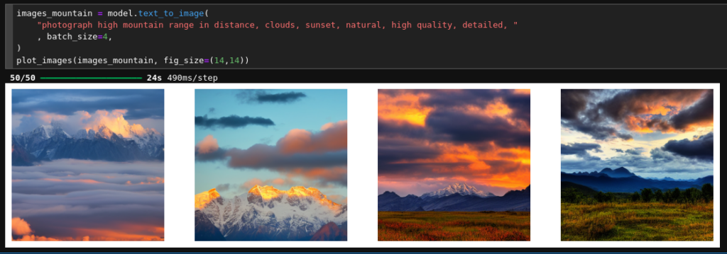
Cell 8 – Testing run: Create Image with mountain range
images_mountain = model.text_to_image(
    "photograph high mountain range in distance, clouds, sunset, natural, high quality, detailed, "
    , batch_size=4,
)
plot_images(images_mountain, fig_size=(14,14))
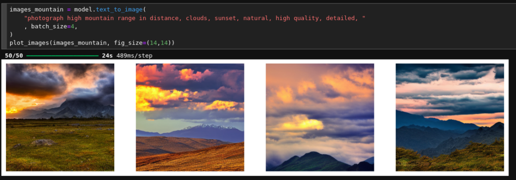
You see that prompting is very simple. Typical results for the given prompt are :


You see that once the model is compiled and has been run once (warm up!), my TI 4060 needs about
- 6.0 secs per image for the standard model;
- 5.1 secs per image for the V2 model. (4 images take around 20 to 21 secs).
This is by a factor of 3 slower than what the Keras CV Team found for a dedicated Nvidia A100 Tensor core card. But it is still a good enough number to get productive on your own system.
During execution the GPU load goes up to 95% up to 98%. Energy consumption per sec is around 125 – 130 Watt.
Prompting
The rest is prompting and fantasy. E.g.:
images_desert_bat = model.text_to_image(
    "photograph of 2 big flying vampires, spread wings, above desert, dune, big moon above, dark night, bright stars, milky way,  "
    "high quality, highly detailed "
    , batch_size=4,
)
plot_images(images_mountain, fig_size=(14,14))
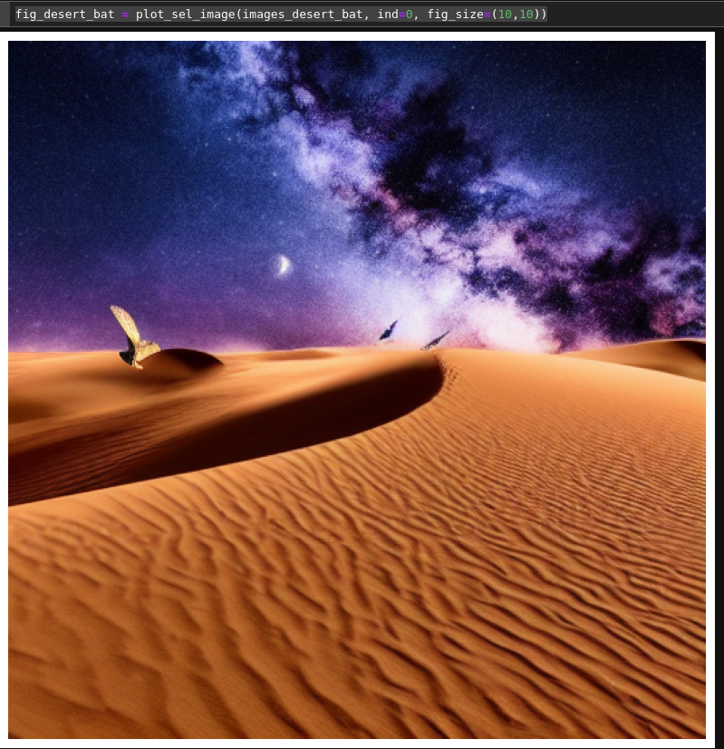
to get:


For the V2 model it may help to use the following prompt: “photograph of flying vampire bats, big spread wings, above a desert, big sand dunes, big full moon rising, very dark night, milky way, fantasy, high quality, highly detailed “.
And when you have created an image you like you can get it in a big single image presentation by
fig_desert_bat = plot_sel_image(images_desert_bat, ind=0, fig_size=(10,10))

The name of the image array must of course be provided correctly. You can save a file with the following command:
fig_desert_bat = plot_sel_image(images_desert_bat, ind=0, fig_size=(10,10))
Now, use your imagination and create reasonable images! You will find that the present diffusion model sometimes has its problems with anatomy – and does not interpret every word in your prompt as you may have meant it. But you will learn quickly how to make your request precise enough …
If you want to put one of the dictators of this world behind prison bars you can e.g. try the following prompt: “NAME_OF_DICTATOR sits on small bed in a long narrow prison cell, grey prison rags, photo “. If the dictator is well known, e.g. because he started a still ongoing war, you may safely assume that he has appeared amongst the training images! But I remind you of the license conditions! Such photo realistic images of persons are only for private consolation that justice one day will prevail!
How does a Diffusion Model for images work? Where can I learn more about it?
Let me briefly summarize my personal understanding of how Diffusion Models for images work. Diffusion in nature is an entropy maximizing statistical process. It transforms a very specific distribution of particles (or other information carrying stuff) slowly but surely into an equilibrium described by a statistical equilibrium distribution. Just think of the development of a drop of ink in a glass of water. Often, the eventual distribution can be described by a multivariate Gaussian. If you want to understand more about statistical distributions occurring in nature please read the very interesting and explanatory publication of S. A. Frank:
S. A. Frank, 2009, “The common patterns of nature“, Journal of Evolutionary Biology, Wiley Online Library.
Regarding an image you have a pixel distribution carrying a lot of specific information. Now imagine that due to some artificial diffusion process the pixel information is spreading into a Gaussian like distribution of pixel noise. In a deterministic world one can approximate such a diffusion process by a quasi-statistic step-wise Markov-chain, with the steps applying a bit of Gaussian noise to the result of the previous step. In the case of a picture you first normalize the pixel information and then – step by step – add a bit of Gaussian noise to the original distribution whilst following restrictions on the mean and the variance.
The nice thing about such a chain of distinct repeated steps is
- that the resulting eventual distribution is almost indistinguishable from real noise,
- but that the progression of the added noise can be described analytically.
Therefore, there is a defined way back to the original image. And for Gaussians the “only” requirement is that an optimal estimation of the mean and the variance of the noise pattern must be made to be able to calculate backwards. The deviation between a given statistical noisy distribution to one generated by a certain Markov chain can be made subject to a Machine Learning process: A neural network can be trained to “guess” the best (analytical) Markov-chain based distribution approximating a given noise pattern – and the respective (probable) original image can be recalculated.
For those of you who are interested in details I recommend to read the important initial publication of J. Sohl-Dickstein, E. A. Weiss, N. Maheswaranathan, S. Ganguli, 2015, “Deep Unsupervised Learning using Nonequilibrium Thermodynamics“.
The second source of information I recommend is the book of D. Foster, “Generative Deep Learning“, 2023, 2nd edition, O’Reilly, Sebastopol, CA, USA. You find both an explanation of Stable Diffusion as well as an example with Keras code in a special chapter on “Diffusion Models” in his very instructive book.
Summary
Thanks to the efforts of the Keras CV team it is possible to run a prompt based image generator model, which uses the Stable Diffusion method, on a consumer PC with a TI 4060. The turnaround times for image creation are in the range of 5 to 6 secs. You need around 8 GiB to run both the standard and the V2 StableDiffusion-models of the Keras CV. The model data are downloaded in h5-format and require more than 3.2 GB each on your disk.