The work on this post series has been delayed a bit. One of my objectives was to use background jobs to directly redraw or to at least trigger a redrawing of Matplotlib figures with backends like Qt5Agg. By using background jobs I wanted to circumvent a blocking of code execution in other further Juypter notebook cells. This would to e.g. perform data analysis tasks in the foreground whilst long running Python jobs are executed in the background (e.g. jobs for training a ML-algorithm). This challenge gave me some headache in the meantime. I just say one word which tells experienced Python PyQt and Matplotlib users probably enough: thread safety.
In this post series we focus on the QtAgg backend first. Well, I found a thread safe solution for dynamic plot updates from background jobs in the context of Jupyterlab and QtAgg. But it became much more complicated than I had expected. It involves a combination of PyQT and Matplotlib. For anything simpler than that you as the user, who controls what is done in a notebook, have to be very (!) cautious.
A growing nest of problems which have to be solved
There are some key problems which we must must solve:
- Interactive mode of Matplotlib with the Qt(5)Agg-backend does not support automatic dynamic canvas updates of Matplotlib figures.
- Interactive mode together with Qt(5)Agg has negative side effects on the general behavior of Python notebooks in Jupyterlab.
- Jupyterlab/IPython has to use its CPU time carefully and must split it between user interactions and GUI processing. This splitting is done in the controlling (event based) loop of your Jupyter notebook, i.e. in the main thread. Whatever other background threads you may start … It is the main loop there which controls the Matplotlib backend interaction with the GUI-data-processing for screen output and the Matplotlib handling of events that may have happened on the displayed figure (GUI-Loop).
- Most GUI related frameworks like PyQt and Matplotib (e.g. with a QtAgg-backend) are not thread safe. It is pretty easy to crash both Matplotlib and PyQt related jobs by firing certain update command to the same figure from two running threads.
- Drawing actions of very many of the so called Matplotlib “artists” and other contributors to continuous updates of Matplotlib figures and as well as of PyQt elements most often must take place in the main thread. In our case: In the main loop of Jupyterlab, where you started your Matplotlib figures or even a main PyQT-window on your (Linux) desktop.
- The draw commands must in almost all practically relevant cases be processed sequentially. This requires a blocking communication mechanism between threads. Otherwise you take a risk of race conditions and complicated side-effects, which all may lead to errors and even may even crash of the IPython kernel. I experienced this quite often the last days.
- Starting side tasks with asyncio in the main asyncio loop of the Jupyter notebook will not really help you either. In some respects and regarding Matplotlib or PyQt asyncio jobs are very comparable to threads. And you may run across the same kind of problems. But I admit that for a careful user and only synchronized requests you may get quite a long way with asyncio. We will study this on our way.
This all sounds complicated – and it indeed is. But you need not yet understand all of the points made above. We have to approach a working Qt5-based solution for non-cell-blocking Python plot jobs in the background of a Juypterlab notebook step by step over some more posts. And I hope your knowledge will grow with every post. 🙂
Topics of this post
In the current post we will use the QtAgg-backend to display Matplotlib Qt5-windows on a (KDE) Linux desktop.
Note: Using “QtAgg” is the preferred mode of invoking the Qt5/6 backend. See the code below. It translates to the available version, in my case to “Qt5Agg“. I therefore will use the term Qt(5)Agg below.
We will try to update two Matplotlib figures, each in its own Qt5-window, and their sub-plots dynamically from one common loop in a notebook cell. Already this simple task requires special commands as Matplotlib’s interactive mode is only partially supported by Qt(5)Agg. In addition we will also come across a dirty side effect of QtAgg on the general behavior of notebooks in Jupyterlab 4.0.x.
Level of this post: Beginner. Python3, Jupyterlab and Matplotlib should be familiar. And you, of course, work with Linux …
Windows for Matplotlib figures outside Jupyterlab and the browser?
If you work as a non-professional in the field of Machine Learning the probability is high that you use Jupyterlab with Python3 notebooks as a convenient development environment. In the first post of this series I have listed up some relevant Matplotlib graphics backends which we can use within Jupyterlab to dynamically update already existing plot figures with graphical representations of new or changed data. A practical application in the context of Machine Learning is e.g. to update plots of metric and other data in your own way during the training of Artificial Neural Networks [ANNs].
While you may be used to display Matplotlib graphics inside a Jupyter notebook (as the output of a certain cell) it may be much more convenient to get a visualization of continuously changing information in (Linux) desktop windows outside the notebook, well, even outside the browser. You may want such external windows even if you accept that the Python code executed in a notebook cell is blocking the use of other cells before all cells commands have been executed.
One reason could be that during ML training runs or other long calculation periods you may want to minimize your Jupyterlab window and work with another application. Another situation could be that the graphics window shall be updated from multiple background tasks of your notebook. Or you may just want to avoid scrolling forth and back in your notebook.
This post shows how we can use the Matplotlib Qt5-backend on a Linux/KDE system for this purpose. The basic idea is to support relatively fast changes of plot figures which are independently placed on the KDE screen outside the Jupyterlab interface in a browser.
Objectives of this post
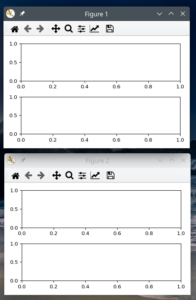
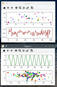
The following graphics illustrates our wishes. It shows two Qt5 windows aside a browser window with a Jupyterlab tab.
The Qt5-windows contain figures with sub-plots (axis-frames). All sub-plots show different data series. All displayed data will later change with some frequency – we want to get a periodic update of the plots from a common update loop. All in all we will study the following aspects:
- Creation of the external windows on the desktop with Matplotlib and Qt(5)Agg.
- Initially filling and singular updates of the sub-plots with the help of code from various notebook cells.
- Periodical update of all figures and their subplots from a common loop in a notebook cell.
Below I will discuss the necessary steps with the help of a simple example.
Obstacle – no intermediate plot updates with the QtAgg backend despite ion()
A quick test shows: The Qt(5)Agg-backend does not react as expected to an enabled “interactive mode” of Matplotlib. To turn “interactive mode” on or off we just have to use the functions pyplot.ion() and pyplot.ioff(), respectively.
In the 1st post of this series we have seen that in interactive mode plot figures, including their canvasses (!), should be updated automatically. At least in a hard interpretation of what is officially published for interactive mode. Presently, this is unfortunately not the case for the Qt5-backend. This does not mean that the ion()-statement is completely superfluous. It guarantees at least that a new figure is automatically shown when the code in a notebook cell finalizes. But it is not sufficient:
The canvas regions of figures and their subplots are not updated automatically.
Below I will demonstrate a workaround and show how we can update multiple plots from a common loop in a notebook cell of Jupyterlab. Such a foreground job in a Jupyterlab notebook is, of course, blocking the execution of code in other notebook cells. I.e. you will not be able to use other cells of your notebook until the present cell’s commands have all been executed. But let us go through the code of an example.
A walk through some example code
Cell 1 – Imports
We need the following imports:
import time
import gc  # need some garbage collection
import sys # for PyQt5
import numpy as np

import matplotlib.backends
import matplotlib.pyplot as plt
from matplotlib.figure import Figure
Cell 2 – Preparation of some plot data
We prepare some objects. The will contain data we can use later on to produce some fancy plots.
# Color list
li_col = ['blue', 'red', 'orange', 'green'
          , 'darkgreen', 'darkred', 'magenta', 'black']
print("Colors prepared")

# Matrics with random data
m_matrix = 200
n_matrix = 100
matrix1 = np.random.normal(0, 1, m_matrix*n_matrix)
matrix1 = matrix1.reshape(m_matrix, n_matrix)
matrix2 = np.random.normal(0, 1, m_matrix*n_matrix)
matrix2 = matrix2.reshape(m_matrix, n_matrix)
matrix3 = np.random.normal(0, 1, m_matrix*n_matrix)
matrix3 = matrix3.reshape(m_matrix, n_matrix)

print("Matrices with random data prepared")

# Array for basic sin function
sin_x = np.arange(0, 2*np.pi, 0.01) # x-array
sin_y = np.sin(sin_x)
print("Basic sin-curve values sin_x/sin_yprepared")

# scatter points
np.random.seed(3)
x_scatter = 4 + np.random.normal(0, 9, 24)
y_scatter = 4 + np.random.normal(0, 2, len(x_scatter))
# size and color:
sizes_scatter = np.random.uniform(15, 80, len(x_scatter))
colors_scatter = np.random.uniform(15, 80, len(x_scatter))
print("scatter points prepared")

# backends
d_backend_list = {'QtAgg':'QtAgg', 'Qt5Agg':'Qt5Agg', 'Gtk3Agg':'Gtk3Agg',
                'TkAgg':'TkAgg', 'ipympl':'ipympl'}
print("dict of backends prepared")
print()
Cell 3 – enforcing the Matplotlib backend
How a certain Matplotlib backend can be enforced was already discussed in the 1st post.
b = d_backend_list['QtAgg']
matplotlib.use(b,  force=True)
# plt.switch_backend(b)
print(" Backend ", b, " enforced")
We invoke our QtAgg backend via matplotlb.use(). The commented variant with switch_backend() also works well, but it will soon get outdated. Note that different backends cannot be used or changed easily in one and the same notebook. When you switch the backend the notebook’s kernel should be restarted.
Hint: For Qt5Agg (and TkAgg), please, do not set ion() already here. It would destroy the functionality of interactive control buttons on the figure windows later. (However, for Gtk3 this setting is required; this will be discussed in another post.)
Cell 4 – Activating interactive mode
We now activate interactive mode via ion():
# Required to ensue working control buttons of the figure windows
# and a direct display of the figure windows
#    If b_ion_on=False you will have to use plt.pause(0.1)
#    or to flush to GUI (see below) to make the figure window visible

b_ion_on = True
if (b == 'QtAgg' or b == 'TkAgg') and b_ion_on:
    plt.ion()
    print(b, "=> ion() and window control buttons activated")
For Qt5 and Tk this statement is required – as long as we do not know better. It ensures that a figure window is displayed on the Linux screen and that the figure’s canvas contents is at least updated as soon as the code of a notebook cell has finished execution. It further ensures the functionality of the Qt-windows’ standard control buttons (e.g. for zooming into the plot).
Cell 5/6 – opening two qt5-windows on the desktop for two figures
fig_1 = plt.figure(num=1,figsize=[5.,3.], clear=True)
fig_1.set_dpi(96.0)
ax11 = fig_1.add_subplot(211)
ax12 = fig_1.add_subplot(212)
fig_1.tight_layout(h_pad = 1)

fig_2 = plt.figure(num=2,figsize=[5.,3.], clear=True)
fig_2.set_dpi(96.0)
ax21 = fig_2.add_subplot(211)
ax22 = fig_2.add_subplot(212)
fig_2.tight_layout(h_pad = 1)

if not b_ion_on:
    plt.pause(0.1)
For Qt5-windows the plt.pause(0.1)-statements are not required if we have switched interactive mode on. But plt.pause does no harm either. plt.pause() would open and show the windows, in a non-blocking way. Even if ion() has not been used.
Keep in mind:
To get Qt-windows on your Linux desktop without having activated interactive mode, just use plt.pause(time), with time being a small interval in secs which you can define with a float.
Both figures have two sub-plots which we will fill later with data. The figure windows should open in KDE at the preferred position for new windows, probably at the center of your (primary) screen.
Watch out that you do not accidentally cover the figures by other windows (watch your Linux desktop’s window information bar, too). Move the windows to a free area of your desktop.
We have achieved our first objective: We have plot-windows outside the browser with our Jupyterlab notebook. And as the standard control-buttons are working, we can even zoom into plots, change settings and save the plots whenever we like to. But to do such funny things we need some canvas contents first.
Cell 7 – update the plot figures once from a single cell
The code below has a parameter b_redraw which is set to b_redraw=False in the beginning. We ignore b_flush completely for some minutes. You will understand its effect later. But feel free to experiment …
# Enforce redrawing of a figures canvas or not
# plt.ioff()
b_redraw = False
b_flush = False

# Update figure 1
# ~~~~~~~~~~~~~~~~
ax11.clear()
ax12.clear()
if b_redraw:
    fig_1.canvas.draw()
    if b_flush:
        fig_1.canvas.flush_events()
    time.sleep(2)

# Just a line plot
col_rand = np.random.randint(0, len(li_col))
i_rand = np.random.randint(0, m_matrix)
ax11.plot(matrix1[i_rand,:], color=li_col[col_rand])

# scatter some points
x_scatter = -3 + np.random.normal(0, 9, 30)
y_scatter = -3 + np.random.normal(0, 3, len(x_scatter))
sizes_scatter = np.random.uniform(15, 80, len(x_scatter))
#colors_scatter = np.random.uniform(5, 50, len(x_scatter))
colors_scatter = np.random.rand(len(x_scatter),3)
ax12.scatter(x_scatter, y_scatter
             , s=sizes_scatter, c=colors_scatter)

if b_redraw:
    st = time.perf_counter()
    fig_1.canvas.draw()
    et = time.perf_counter()
    rt = et - st
    print("time spent for redrawing fig 1: ", '%.3f' %rt)
    if b_flush:
        fig_1.canvas.flush_events()
    time.sleep(1)


# Update figure 2
# ~~~~~~~~~~~~~~~~
ax21.clear()
ax22.clear()
if b_redraw:
    fig_2.canvas.draw()
    if b_flush:
        fig_2.canvas.flush_events()
    time.sleep(2)

# scatter more points
x_scatter = 4 + np.random.normal(0, 9, 150)
y_scatter = 4 + np.random.normal(0, 3, len(x_scatter))
sizes_scatter = np.random.uniform(15, 80, len(x_scatter))
#colors_scatter = np.random.uniform(9, 30, len(x_scatter))
colors_scatter = np.random.rand(len(x_scatter),3)
ax21.scatter(x_scatter, y_scatter
             , s=sizes_scatter, c=colors_scatter)

# plot a sinus curve
col_rand = np.random.randint(0, len(li_col))
x = np.arange(0, 24*np.pi, 0.01)            # x-array
ax22.plot(x, np.sin(x), color=li_col[col_rand])

if b_redraw:
    st = time.perf_counter()
    fig_2.canvas.draw()
    et = time.perf_counter()
    rt = et - st
    print("time spent for redrawing fig 2: ", '%.3f' %rt)
    if b_flush:
        fig_2.canvas.flush_events()
With b_redraw=False the plot update should work pretty fast – if (and only if) we had set interactive mode on via ion() (see cell 4). If we set b_redraw=True additional commands of the type yourFigure.canvas.draw() are executed.
The “fig.canvas.draw”-command theoretically enforces a re-rendering of the contributions of all artists in the backend (see below and here). In the sense of the “hard” interpretation of Matplotlib’s “interactive mode”, we would expect that the result is directly displayed in our Qt5-windows. Well, let us see ….
We first run our cell 7 with b_redraw=False. Works perfectly. Both plots are updated. So, interactive mode seems to do its job properly. However, our little code executes very fast on a modern CPU. So you cannot see whether e.g. the updates of ax11 ad ax12 really happen before the 2nd figure is updated.
However, we can test the real behavior with setting b_redraw=True. This will not only trigger a re-rendering, but a sleeping interval of 1 sec, too. Then we run the cell code again. Surprise, surprise …
You will experience that none of the draw-requests had any effect on the figure windows! The figures are not even cleared as requested in the beginning. Still, both figures and their sub-plots get updated only when the cell’s code finalizes.
So things are not so simple. Obviously, elementary Matplotlib plot commands followed by a canvas.draw() have no direct effect in our Qt5-windows. It is as if we decouple the commands of a code cell from GUI-processing during execution. Or, more precisely: The results of our commands are not processed in some kind of a GUI-loop which would produce output on the screen before all Python and Matplotlib code in the cell has been executed. Plot output production is done deferred. Even if ion were set.
This appears a bit strange as we would reasonably assume that a render-request via canvas.draw() is actually performed by the backend. And, indeed, we see that it consumes significant CPU-time. The print output of our cell reveals something like this:
time spent for redrawing fig 1:  0.032
time spent for redrawing fig 2:  0.035
This all forebodes nothing good for continuously updating the plots dynamically from a loop. It seems that we either are stuck or that we need additional commands to ensure that the results of our explicit canvas.draw()-requests really reach the output engine of our Linux GUI such that the backend’s render results get displayed on the screen.
Interestingly, it seems that we do not need the yourFigure.canvas.draw() commands if we can await the cell’s code end. Hmm .., is this really true?
Well, we do not need canvas.draw()-commands if interactive mode was switched on. You can test this easily with executing a plt.ioff() at the beginning of cell 7 and rerunning the code with b_draw=False. Then, nothing gets updated at all. Ufff ….
Intermediate results
- With non-interactive mode [set via ioff()] “yourFigure.canvas.draw()“-commands are required for all of your figures to enforce canvas updates. But the updates are done only when the notebook cell’s code execution has finished.
- With interactive mode [set via ion()] “yourFigure.canvas.draw()“-commands are not required. Obviously, ion() ensures that all redraw commands are executed for all (or all affected) figures (+ something else).
- Problem: Even with interactive mode activated a command “yourFigure.canvas.draw()” will not lead to a canvas update until the cell code’s command sequence has finalized. Only then we seem to get a connection to the full GUI-processing loop again.
Note: One would not complain about this kind of working of the interactive mode if there were not other backends which do provide a direct and automatic updating of the figures canvas region after having requested yourFigure.canvas.draw(). One example is the “ipympl”-backend. Any graphic output of ipympl is however displayed within the Jupyterlab interface.
Now, let us see what the consequences for loops in notebook cells are.
Cell 8 – a function to update the figures/sub-plots periodically within a Python loop
With the next plot we prepare a more profound test. The function will try to update our figures continuously.
def common_update_loop(ax11, ax12, ax21, ax22, li_col
                       , b_flush=False
                       , b_draw=False, b_draw_idle=False
                       , sleep_time=0.005
                       , n_chg=81
                      ):
    j = 0
    start_time = time.perf_counter()
    for i in range(0, n_chg):
        if i == 2:
            st_in1 = time.perf_counter()
        if i == n_chg-1:
            st_in2 = time.perf_counter()

        # output
        if i%20==0:
            print(i)
        if j%8 == 0:
            j = 0

        # Fig 1/1 - update
        ax11.clear()
        x_scatter = 4 + np.random.normal(0, 9, 30)
        y_scatter = 4 + np.random.normal(0, 3, len(x_scatter))
        sizes_scatter = np.random.uniform(15, 80, len(x_scatter))
        #colors_scatter = np.random.uniform(5, 50, len(x_scatter))
        colors_scatter = np.random.rand(len(x_scatter),3)
        ax11.scatter(x_scatter, y_scatter
                     , s=sizes_scatter, c=colors_scatter)

        # Fig 1/2 - update
        ax12.clear()
        col_rand = np.random.randint(0, len(li_col))
        ax12.plot(matrix2[i,:], color=li_col[col_rand])
        if b_draw:
            if not b_draw_idle:
                fig_1.canvas.draw()
            else:
                fig_1.canvas.draw_idle()
        if b_flush:
            fig_1.canvas.flush_events()

        # Fig 2/1 - update
        ax21.clear()
        col_rand = np.random.randint(0, len(li_col))
        x = np.arange(0, i*np.pi, 0.01)
        ax21.plot(x, np.sin(x), color=li_col[j])

        # Fig 2/1 - update
        if i == 3:
            st_in10 = time.perf_counter()
        ax22.clear()
        if i == 3:
            et_in10 = time.perf_counter()

        if i == 3:
            st_in5 = time.perf_counter()
        if i == n_chg-1:
            st_in3 = time.perf_counter()

        x_scatter = 4 + np.random.normal(0, 9, 150)
        y_scatter = 4 + np.random.normal(0, 3, len(x_scatter))
        sizes_scatter = np.random.uniform(15, 80, len(x_scatter))
        #colors_scatter = np.random.uniform(9, 30, len(x_scatter))
        colors_scatter = np.random.rand(len(x_scatter),3)
        ax22.scatter(x_scatter, y_scatter
                     , s=sizes_scatter, c=colors_scatter)
        if i == 3:
            et_in7 = time.perf_counter()

        if i == 3:
            st_in8 = time.perf_counter()
        if b_draw:
            if not b_draw_idle:
                fig_2.canvas.draw()
            else:
                fig_2.canvas.draw_idle()
        if i == 3:
            et_in8 = time.perf_counter()

        if i == 3:
            et_in5 = time.perf_counter()
        if i == n_chg-1:
            et_in3 = time.perf_counter()

        # flushing and rspective timing
        if i == n_chg-1:
            st_in4 = time.perf_counter()
        if i == 3:
            st_in9 = time.perf_counter()
        if b_flush:
            #fig_1.canvas.flush_events()
            fig_2.canvas.flush_events()
        if i == 3:
            et_in9 = time.perf_counter()
        if i == n_chg-1:
            et_in4 = time.perf_counter()

        # color update
        j += 1

        if i == 2:
            et_in1 = time.perf_counter()
        if i == n_chg-1:
            et_in2 = time.perf_counter()

        # wait a bit
        time.sleep(sleep_time)

    print("finished")

    # some timings
    end_time = time.perf_counter()
    cpu_time = end_time - start_time
    it = (et_in1 + et_in2 - st_in1 - st_in2) / 2.
    print()
    theor_time = (it + sleep_time) * n_chg
    print("Loop  time: ", '%.2f' %cpu_time
          , " :: it =", '%.3f' %it)
    print("Theo. time: ", '%.2f' %theor_time
          , " :: it =", '%.3f' %it )
    t_prep_ax = et_in3 - st_in3
    t_flush = et_in4 - st_in4
    print("CPU time data prep: ", '%.4f' %t_prep_ax
          , " :: flush time =", '%.5f' %t_flush )

    # all times for i=3
    t_prep_ax_22   = et_in5 - st_in5
    t_clear_ax_22  = et_in10 - st_in10
    t_calc_ax_22   = et_in7  - st_in5
    t_draw_ax_22   = et_in8  - st_in8
    t_flush_ax_22  = et_in9  - st_in9
    print()
    print("i=3:")
    print("clear time ax22 : ", '%.5f' %t_clear_ax_22)
    print("calc  time ax22 : ", '%.5f' %t_calc_ax_22)
    print("draw  time fig2 : ", '%.5f' %t_draw_ax_22)
    print("prep  time ax22 : ", '%.5f' %t_prep_ax_22)
    print("flush time fig2 : ", '%.5f' %t_flush_ax_22)
    return
Take your time to study the code. Ignore the difference between using canvas.draw_idle() and canvas.draw() for the rest of this post. I will come back to it in the next post.
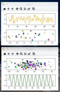
The eventual result of this function is displayed in the image. ax11 and ax22 are updated with changing scatter-plots. ax12 displays a changing signal plot, ax21 a sinus-curve whose period should become shorter with time.
The period by which the loop’s commands are executed is determined by a parameter sleep_time.
We also measure the required CPU-time to perform an update at two defined iterations – the 2nd and the last. This allows us to find out whether the loops duration is dominated by sleep_time or the execution time for the data preparation and plot updates.
During iteration 3 we also measure detailed time intervals for the execution of all steps executed to update the contents of ax22.
Note also that the parameter b_flush controls the activation of a new command, namely
yourFigure.canvas.flush_events()
We will see that this command is a key for a dynamic update of our figures’ canvas areas.
Cells 9 and 10 – clearing the sub-plots and executing the loop with interactive mode on
To get a better impression of what happens we first clear all sub-plots.
plt.ion()
ax11.clear(); ax12.clear(); ax21.clear(); ax22.clear()
Then we start the loop with b_flush=False, b_draw=False and b_draw_idle=False:
plt.ion()
#plt.ioff()
loop_start_time = time.perf_counter()
common_update_loop(ax11, ax12, ax21, ax22, li_col
                   , b_flush=False
                   , b_draw=False
                   , b_draw_idle=False
                   , n_chg=61)
Unfortunately, it takes some time around 3 sec until something happens at all.
If we have cleared all sub-plots by executing cell 9, then the empty canvases are displayed until the cell code execution finalizes.
The print output shows that the total loop time is approximately equal to the measured time required for data creation and plotting multiplied by the number of iterations.
As it should be:
0
20
40
60
finished

Loop  time:  3.16  :: it = 0.044
Theo. time:  2.99  :: it = 0.044
CPU time data prep:  0.0010  :: flush time = 0.00000

i=3:
i=3:
clear time ax22 :  0.01895
calc  time ax22 :  0.00185
draw  time fig2 :  0.00000
prep  time ax22 :  0.00185
flush time fig2 :  0.00000
The time for one iteration is around (0.046+0.005)=0.51 sec, the last summand being the sleep-time. Which fits well for the measured data preparation time for the dominating scatter plot of ax22. The time for the scatter plot in ax11 is similar. They both together make most of the time (2*0.22 sec) of one iteration in the loop of function common_update_loop().
Only after the code in our cell has been executed completely we get a screen update (see the plot besides). At that point we just get a display of the graphical information for the latest set of data prepared. This is, of course, due to the intermediate clear()-requests.
We have once again confirmed for the current version of the QtAgg-backend that ion() itself does not guarantee intermediate plot updates when requested via specific commands in a loop or during code execution in a notebook cell. But direct plot updates would be a minimum requirement for dynamic plotting! Is there a remedy?
Executing the loop with b_flush=False, b_draw=True => canvas.draw() becomes dominant for CPU time
To get an impression of what the yourFigure.canvas.draw()-commands cost in terms of CPU time we rerun the loop, but this time with settings b_flush=False and b_draw=True. Again we do not get intermediate updates, but the total turnaround time grows significantly!
Obviously the time for all the two canvas.draw()-commands becomes the dominant factor regarding CPU time consumption (in our specific example).
0
20
40
60
finished

Loop  time:  8.09  :: it = 0.123
Theo. time:  7.84  :: it = 0.123
CPU time data prep:  0.0544  :: flush time = 0.00000

i=3:
i=3:
clear time ax22 :  0.00604
calc  time ax22 :  0.00109
draw  time fig2 :  0.04728
prep  time ax22 :  0.04836
flush time fig2 :  0.00000
This is not so surprising as it may seem on first sight: Scatter plots do require some extensive calculations in order to perform the rendering right on the pixel level with respect to the overlap of very many extended and rounded elements in our case.
Cell 11 – Executing the loop with b_flush=True
The next cell repeats the loop, but this time with a setting our parameter b_flush=True AND b_draw=True.
common_update_loop(ax11, ax12, ax21, ax22, li_col
                   , b_flush=True, b_draw=True
                   , b_draw_idle=False, n_chg=61)
This time we get the aspired continuous intermediate updates of the plot figures! You can see this in a video below (hoping that your browser supports the format).
The print output is close to the one we got before:
0
20
40
60
finished

Loop  time:  8.09  :: it = 0.130
Theo. time:  8.25  :: it = 0.130
CPU time data prep:  0.0513  :: flush time = 0.00040

i=3:
i=3:
clear time ax22 :  0.00919
calc  time ax22 :  0.00180
draw  time fig2 :  0.06360
prep  time ax22 :  0.06541
flush time fig2 :  0.00029
Note that we now also see a (tiny) amount of time spent for flushing the render results to the backends GUI-loop. Compared to the canvas.draw()– time this flush-time is, however, negligible.
Video of continuous dynamic figure updates
The video was done and reduced in size with the program SimpleScreenRecoder of Maarten Baert. See https://www.maartenbaert.be /simplescreenrecorder/
Now we also see the expected change in period length for the sinus-curve! This proves the continuous updating according to changing plot requests during the iterations of the loop in common_update_loop()’s.
Note that the video was recorded during an interval of all in all 30 iterations. Therefore the period length is shorter than in the image above which was taken after only 20 iterations.
Obviously we have found a proper solution for our problem. But have we understood all of our findings?
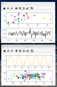
Do the control buttons work?
Just to show you the even control buttons of the Qt-windows are really working I have zoomed into the the sub-plots of figure 2 after yet another run. This is shown in the next graphics:
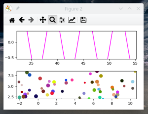
Note the active zoom-symbol. I leave it to the reader to get familiar with the functionality of the other buttons on his/her own.
You can test, by the way, that commands from the control buttons are in principle even respected whilst loop is running. The actions are interfering with the fast clear()-command. But if you use the shift button on one sub-plot you will notice a delay of the updates.
You can also use the “settings button”, change the hspace value there (between 0,0 and 1.0) and press “Enter” while our loop is running. The vertical distance between the sub-plots will change accordingly whilst the ax-frames are continuously updated with new data !
The control buttons are artists (in the sense of Matplotlib) that contribute to plotting of a figure’s canvas. When you run common_update_loop() again with b_flush=False you will see that button related requests to the GUI are deferred until the code of the notebook cell has finalized.
A dirty side effect of ion() with QtAgg on the Jupyterlab notebook
This paragraph was changed on 12/23/2023 to correct some statements.
I had to confirm with some simple tests because I could not believe it: If you use the QtAgg backend your Python notebook will behave unexpectedly strange after some error has occurred in a cell. Afterward you may not be able to run another cell without clicking on the “Run” symbol twice. Also selecting and running multiple cells may behave strange. At least one of the selected cells may stay in a waiting status and will not start. Again you have to click “Run” twice to continue normal working. This is the status of Jupyterlab 4.0.9 run in Firefox. Python kernel 3.9.18.
This is very inconvenient! I found no workaround, yet, except adding a tag “raises-error” to the cell via “Common Tools” in the right side-bar of Jupyterlab. There does not seem to be a general notebook or session-wide option.
Do we need ion()?
Well, as you have learned above, we do not really need ion() to cooperate with QtAgg. Even with interactive mode off, we can always get what we want by using the commands
- plt.pause(0.1) to bring our Qt-windows with the figures onto our desktop
- yourFigure.canvas.draw() followed by yourFigure.canvas.flush_events() to enforce canvas updates
By the way: the second point is not sufficient to get the windows with the figures initially on the desktop screen.
Conclusion
We have achieved our 3 objectives for this post. However, we also got the feeling that Matplotlib’s interactive mode behaves a bit strange when used with the QtAgg-backend. In addition interactive mode changes the behavior of Jupyterlab for cell execution in a very unusual way. So, we would be better off without it.
Fortunately, we have identified and tested commands which bring Qt-windows for our figures onto the Linux desktop and which enable us to perform really dynamic canvas updates when we like them to appear on the screen – during cell code execution! And without interactive mode!
However: I have not yet given any explanation for the result that without the canvas.flush_events()-command plot updates are deferred until all code of a Jupyter cell has been executed. This is the topic of the next post in this series. It will help us to understand a bit better why plot update commands from background jobs will later be handled differently. Stay tuned ….