Quadratic form functions as graph functions – I – level sets and gradients

The last months I have seldom written posts in this blog. The reason is that I am occupied with a book about “The geometry of Multivariate Normal Distributions”. Which will cover a lot more topics than the ones discussed in this blog so far.

One of those topics is the use of quadratic form functions as graph functions to produce hypersurfaces in the ℝⁿ. The level sets of such hypersurfaces are multidimensional ellipsoids in the general case. In this post, however, I want show you some elements of the discussion of 2-dimensional hypersurfaces in the ℝ³ created by quadratic form functions. Respective level sets are ellipses. I will not give any proofs in this article; readers will soon find mathematical derivations in a forthcoming booklet on ellipses and their representation by matrices which I will publish in this blog. Have some patience.

In the realm of Machine Learning, Bivariate Normal Distributions [BVN] characterize data distributions of certain classes of natural objects in their multidimensional feature space or in latent spaces of artificial neural networks. Just as a reminder: The 2-dim projections of the multivariate data distribution in the latent space (with hundreds of dimensions) of a Convolutional Autoencoder trained on human faces approximate BVNs very closely. This reflects a natural correlation of core properties of human faces which follow Gaussian distributions. (Such distributions have an extremal entropy value among statistical distribution controlled by two parameters. Multivariate normal distributions are a natural outcome of evolutionary processes which got an impact of very many factors.)

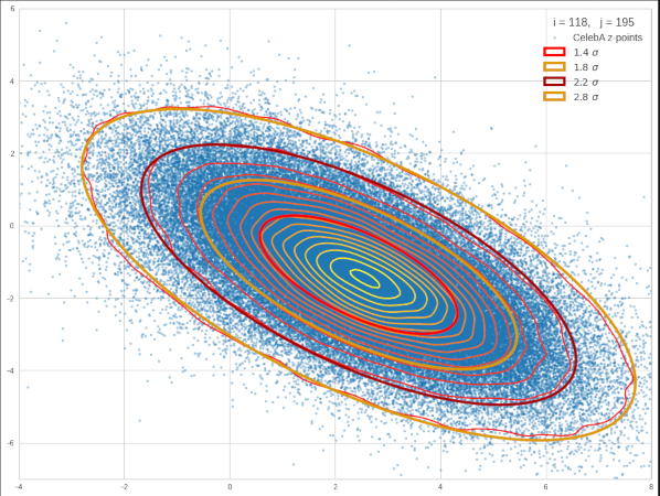
The smooth red line, the darkred line and also the orange line show confidence ellipses based on the numerically determined correlation matrix of the data, the slightly wiggled lines represent numerically determined contours.

For the analysis of such distributions we naturally work with confidence ellipses because they are contour lines of ideal BVNs. But sometimes it is simpler to work with the quadratic form function whose coefficients correspond to the elements of the inverse covariance matrix in the exponent of a BVN.

A warning: For the analysis of real world data of natural objects we should not forget that the covariance matrix itself must be computed numerically from the given data in latent spaces. Such a covariance matrix can always be computed, but its existence is no guarantee for a real multivariate or bivariate distribution inside some core of the centered distribution. Other criteria have to be evaluated, too.

Quadratic form function – and its relation to BVN distributions

Readers of this blog recognize

\[ F_E(x,y)\,=\, \alpha\,x^2 \,+ \beta \,x\,y +\gamma\,y^2 \tag{1} \]

as a function whose level sets

\[ F_E(x,y)\,=\, C_i\,=\, const. \tag{2} \]

define ellipses and whose coefficients α, β and γ are elements of a respective invertible quadratic form matrix:

\[ \pmb{\operatorname{Q}}_E \,=\, \begin{pmatrix} \alpha & \beta/2 \\ \beta/2 & \gamma \end{pmatrix}\,. \tag{3} \]

The relation to BVNs and their confidence ellipses: Such a symmetric matrix appears in a somewhat different form in the exponent of the probability density function g₂(x,y) of a BVN. See e.g. this post and this one.

\[ g_{2}(\mathbf{x})\,=\, {1 \over 2\,\pi\,|\mathbf{\Sigma}|^{1/2}\,}\,\exp\,\left[-\frac{1}{2}\left(\pmb{\operatorname{x}}^{\mathsf{T}}\circ\mathbf{\Sigma}^{-1}\circ\pmb{\operatorname{x}}\right)\right]\,,\quad\text{with}\,\,\,\pmb{\operatorname{x}}\in\mathbb{R}^{2}\,. \tag{4} \]

\[ \begin{align} \mathbf{\Sigma}\,=\,Q_{\mathsf{E}}^{\mathsf{-1}}\,& =\:\begin{pmatrix}\sigma_{x}^{2} & \rho\,\sigma_{x} \sigma_{y}\,\\ \,\rho\,\sigma_{x} \sigma_{y} & \sigma_{y}^{2} \end{pmatrix} \tag{5} \\[10pt] \mathbf{\Sigma}^{-1} \,=\,\mathbf{Q_{\mathsf{E}}}\,&=\, {1 \over \sigma_{x}^{2}\,\sigma_{y}^{2}\,\,(1-\rho^{2})}\:\, \begin{pmatrix}\sigma_{y}^{2} & -\rho\,\sigma_{x}\,\sigma_{y}\\ -\rho\,\sigma_{x}\,\sigma_{y} & \sigma_{x}^{2} \end{pmatrix} \tag{6} \end{align} \]

Of course, there exists a transformation between the coefficients α, β and γ and the BVN parameters σ_x, σ_y and the Pearson correlation coefficient ρ of a BVN:

\[ \begin{align} \sigma_{x}\, &=\,\left[ {4\,\gamma} \over {4\,\alpha\,\gamma-\beta^{2} } \right]^{1/2}\,, \\[10pt] \sigma_{y}\, &=\,\left[ {4\,\alpha} \over {4\,\alpha\,\gamma-\beta^{2} } \right]^{1/2}\,, \\[10pt] \rho\,\, &=\,-\frac{1}{2}\, {\beta \over \sqrt{\alpha\:\gamma\,} }\,. \end{align} \tag{7} \]

and, reversely,

\[ \begin{align} \alpha\, &=\, {1 \over \sigma_x^2 \,( 1\,-\, \rho^2) }\,, \\[10pt] \gamma\, &=\, {1 \over \sigma_y^2 \,( 1\,-\, \rho^2) }\,, \\[10pt] \beta\, &=\,-\, {2 \rho \over \sigma_x \,\sigma_y \, (1 – \rho^2)} \,. \end{align} \tag{8} \]

Readers can deduce these relations from previous posts in this blog or wait for a booklet on ellipses and their matrix representation, which I am going to provide soon. BVNs incorporate quadratic form matrices in a certain parameter notation.

We have analyzed matrices of the types Q_E and Σ already a lot in this blog. Most of the time with the toolset of Linear Algebra. Under the assumption that the matrix elements guarantee positive-definiteness, the eigenvalues give us the lengths of the semi-axis of an ellipse corresponding to

\[ F_E(x,y) \,=\, 1\,, \quad \pmb{\operatorname{x}}^{\mathsf{T}}\circ\mathbf{\Sigma}^{-1}\circ\pmb{\operatorname{x}} \,=\, 1\,, \tag{9} \]

and the eigenvectors define the direction of the semi-axes. Scaled versions of this ellipse are not only level sets of F_E, but also of the related BVN. We have seen in previous posts that concentric ellipses with the same ratio of their major to minor semi-axes can be generated by either using a different constant C ≠ 1 – or by dividing the coefficients α, β and γ by some constant C.

Something which we have not done so far is to regard F_E (x,y) as a graph function in the ℝ³ and/or as a scalar function defined on an open set of the ℝ² with 1-dimensional level sets. By taking these points of view, we can employ a lot of insights from multivariate calculus.

The quadratic form function as a graph function

Very simplified, a graph is a continuous set of vectors defined by a parameterization on some open set of a lower dimensional sub-space. In our case we create a 2-dim hypersurface S_F based on a parameterization of the following form

\[ \begin{align} \text{graph}(F_{E})\,=\, S_F \, &:=\,\left\{ \:\mathbf{x}_{S}\,=\,(x,y,z)\quad|\quad\mathbf{v}=(x,\,y)^{\mathsf{T}}\in\mathsf{U},\,\:\mathsf{U}\subset\mathbb{R}^{2}\,\,\land\,\,z=F_{E}(\mathbf{v})=F_{E}(x,y)\,\right\} \,,\\&=\,\left\{ \:\left(x,y,F_{E}(x,y)\right)\,\,|\,\:(x,\,y)^{\mathsf{T}}\in\mathsf{U}\,\right\} \end{align} \,. \tag{10} \]

U is an open set around the origin of a Cartesian coordinate system [CCS] covering the ℝ² . F_E(x,y) is used as a graph function which depends on the two parameters x and y. The resulting hypersurface is shown in the illustration below

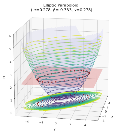
hypersurface of a paraboloid created by a quadratic form function

I have indicated a level set of this hypersurface at z = 2 by red points and other level sets given by

\[ F_E(x,y) \,=\, C_i = const., \quad \text{with} \,\,\, 0 \lt C_i \le 5.5 \,. \tag{11} \]

by colored curves. These level sets are created by cutting the surface with planes that are parallel to the (x,y)-plane. In addition, the projections of the level sets on the (x,y)-plane are shown. As expected, we get a bunch of concentric ellipses. (The plot itself was created with the help of Matplotlib 3D, its “surface”- and contour-functions and meshgrids.)

We understand why the shown surface is called an elliptic paraboloid: Its dimensions at a level z=C are given by the semi-axes of the respective contour ellipse.

Level sets of the quadratic form function and graph functions of the ellipses

Both a BVN’s probability density function g₂(x,y) as well as the respective quadratic form function F_E (x,y) give us concentric ellipses as level sets. Vector analysis tells us via the “Implicit Function Theorem” that every level set can locally be represented by a graph function (which is implicitly defined). Multiple graph functions may be needed to fully cover a level set’s curve (or surface).

In our rather simple case the ellipses are represented by two 1-dim graph functions:

\[ y_{U/L}(x,C)\, =\:{1 \over 2\,\gamma} \: \left(\,-\,\beta\,x\, \pm \, \left[\,4\,\gamma\,C\,-\,\left(4\,\alpha\,\gamma-\beta^{2}\right)\,x^{2}\,\right]^{1/2}\,\right)\,, \]

which are defined on the same interval for x-values. The condition for the limits of this interval is that the square root argument must be positive. (I leave the question of a proper orientation of the resulting curves for the time being to the reader).

All well known properties of ellipses can in principle be derived from these functions. (Sometimes, this may turn out to be harder than expected; see a previous post in this blog for an example.) However, for finding normal vectors perpendicular to the respective elliptic curves it is easier to employ the “mother” function F_E(x,y), which we have used as a graph function itself. We just have to determine its gradients and can avoid differentiating y_U/L(x) with its square root.

Gradient vectors – perpendicular to the hypersurfaces of elliptic level sets

A well known insight of vector analysis tells us that the gradients of a scalar function F(x):ℝⁿ→ℝ are vectors perpendicular to the contour surfaces (or curves) given by level sets of function F(x). Actually, in our case, this gives rise to a 2-fold sequence of gradient vectors.

First it is easy to understand that the surface S_F created by F_E can be regarded as a level set of a scalar function Ψ(x,y,z) defined on an open set of the ℝ³

\[ \Psi(x,\,y,\,z) \,=\, \alpha\,x^2 \,+ \beta \,x\,y +\gamma\,y^2 \,-\, z \,, \tag{12} \]

namely for a constant C=0:

\[ \Psi(x,\,y,\,z) \,=\, \alpha\,x^2 \,+ \beta \,x\,y +\gamma\,y^2 \,-\, z \, =\, C\,=\, 0,\quad \Rightarrow \quad S_F \,=\, \Psi^{-1} (0) \,. \tag{13} \]

This means that the gradient vector ∇Ψ(x,y,z) should be a normal vector perpendicular to S_F at any points (x,y,z) ∈ S_F :

\[ \nabla \,\Psi(x,y,z) \,=\, \begin{pmatrix} 2\,\alpha\,x \,-\, \beta\, y \\ 2\,\gamma\,y \,-\, \beta\, x \\ -1 \end{pmatrix} \,\perp\, S_F, \quad \,\text{at any} \,\, (x,y,z) \in S_F \,. \tag{14} \]

The following plot indicates this:

Normal vectors of a quadratic form function's paraboloid

The plot was done with Matplotlib and the “FancyArrowPatch”. [Hint: To get the orientation of the vectors right, you must take into account the scaling of the axes. In addition you should use ax.set_proj_type(‘ortho’)].

Note that “orthogonality” to a surface at a point with position vector x=(x,y,z) actually means that the normal vector n must be perpendicular to all of those curves within S_F that pass through x. The orthogonality to a curve in turn is defined by a zero scalar product of n with the tangent vector t to the curve at point x: n • t = 0.

Gradients to the 2-dim hypersurface

We can see the orthogonality much more clearly by moving into the main axis system of a given elliptic paraboloid. I.e., we choose a new CCS such that the axes of the elliptic levels get aligned with axes of this CCS. The respective rotation of the CCS affects the quadratic form coefficients: We get a value of β=0 for the axis-parallel paraboloid in the rotated CCS.

The next plot shows gradient vectors derived from ∇Ψ(x,y,z) and tangents to the surface at border points of an elliptic paraboloid whose symmetry axes got aligned with the coordinate axes of the chosen CCS:

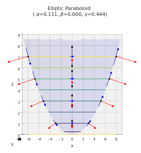
Normal and tangent vectors at border curves of a paraboloid

And for the other extension in y-direction:

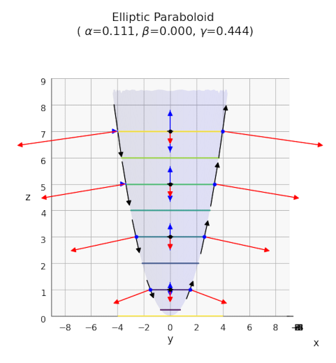
The limiting curves at the borders of the axis-parallel paraboloid in x– and y-direction are, of course, parabolas. In general we find that coordinate lines on the paraboloid, i.e. curves for which we keep either x or y constant, are parabolas. We will see this graphically a bit better in the next post of this series when we will discuss tangent vectors.

The gradient vectors (in red) and tangent vectors (in blue or black) were scaled by different constant factors to avoid a clattering of vectors. We clearly see the orthogonality of the gradient vectors with respect to the paraboloid’s surface now. The variation of the lengths of the gradient vectors follows directly from their dependence on x and y.

For the reader it could be instructive to prove the orthogonality mathematically. (You will find such a proof in my forthcoming booklet on ellipses.)

Gradients of the quadratic form function orthogonal to the elliptic level sets

The ellipses given by level sets of F_E(x,y) are elliptic contour curves resulting from cutting the graph S_F by surfaces parallel to the (x,y)-plane. The 2-dim gradient vectors of F_E(x,y) are composed of the x– and y-components of the gradients of Ψ(x,y,z):

\[ \nabla \,F_E(x,y) \,=\, \begin{pmatrix} 2\,\alpha\,x \,-\, \beta\, y \\ 2\,\gamma\,y \,-\, \beta\, x \end{pmatrix} \,. \tag{15} \]

These gradients must be perpendicular to the F_E‘s level sets – i.e. to our ellipses and the curves created by their graph functions.

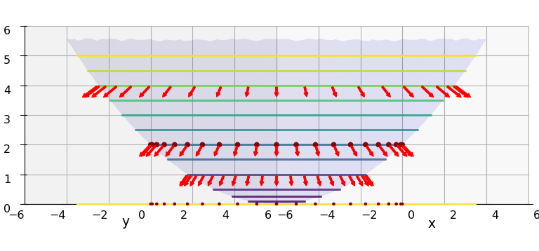
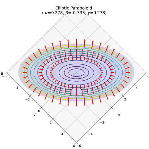
This means that a view along the z-axis of the paraboloid shown in the first plot and thus vertically upon the gradient vectors of the mother function Ψ (attached at selected points) should show us vectors perpendicular to the projected ellipses. The following plot produced with Matplotlib for an elevation angle of π/2 shows the expected result (for an azimuth angle of π/4):

Orthogonal projection of paraboloid, its contour ellipses and related normal vectors

For yet another ellipsoid I got the following results (derived with different methods and different scalings):

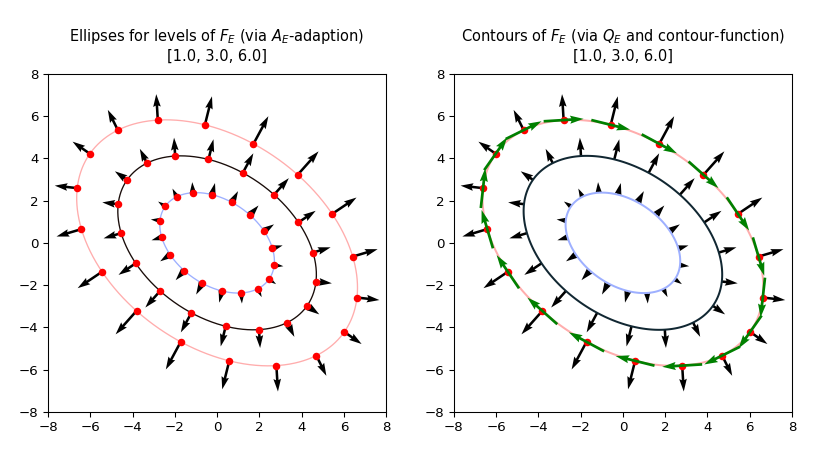
ellipses from quadratic form and normal vectors

The right plot shows tangential vectors in addition. The orthogonality is striking again.

The reason that the gradient vectors are longer for the elongated side of the ellipse is that the contours of F_E are much denser vertical to the major axis than on the side of the minor axis.

Conclusion and outlook

Studying the role of the quadratic form function of ellipses as a graph function in the ℝ³ also expands our view on BVNs. We can regard a BVN’s confidence ellipses as level sets of a quadratic form function with properly chosen coefficients derived from the BVN’s covariance matrix.

The elliptic curves of the resulting level sets are clearly seen in 3D presentations of the hypersurface generated by F_E(x,y) in the ℝ³. We found that the hypersurface is an elliptic paraboloid with (at least some) coordinate curves on its surface being parabolas.

The existence of two graph functions which constitute a closed contour ellipse on an interval along the x-axis is guaranteed implicitly by the quadratic form function F_E. Normal vectors of the concentric contour ellipses can be calculated as gradient vectors of F_E(x,y).

The reader knows of course that vectors perpendicular both to the surface created as the graph of F_E(x,y) as well as to the closed ellipses can also be constructed from tangent vectors. Another interesting question is whether and how the Gaussian curvature of F_E‘s hypersurface is related to the curvature of its contour ellipses. We will investigate both points in forthcoming posts. Stay tuned ….