Covariance matrix of a cut-off Multivariate Normal Distribution – I – intricate integrals with exponentials over the volumes and surfaces of n-dimensional ellipsoids?

In Machine Learning and statistics one sometimes has to work with a data sample whose underlying probability distribution approximates a Multivariate Normal Distribution [MVN] – but only within the ellipsoidal region of an innermost core with limited extensions. I.e., we have a MVN which either is abruptly cut off at some finite Mahalanobis distance D, or which quickly changes into another (asymmetrical) kind of distribution beyond this distance. Given such a situation: How can we use the sample’s data to estimate the covariance matrix of the MVN, which appears to controls the statistical distribution inside the core?

Our sample may provide us with a sufficient number of data points residing inside our identified core. Then, we may throw away all disturbing data points outside the core and perform an analysis of the core’s MVN-like distribution, only. In particular, we would like to get a good estimate of the covariance matrix of the core region and of the respective original MVN.

Unfortunately, a sample of data points which reside inside inside an ellipsoidal core region of a MVN does not give us a direct clue about the values of the elements of the covariance matrix of a respective infinite MVN. I will first show this with the help of some examples and afterwards prove it via a mathematical analysis.

Actually, we need to find a reliable mathematical relation between the covariance matrix (numerically) determined for a limited core region of a cut-off MVN on the one hand side, and the elements of the covariance matrix of the respective infinitely extended MVN on the other hand side. We expect such a relation to depend strongly on the limiting Mahalanobis distance D.

This challenge appears to be a simple one at first sight. However, when you start to tackle the required mathematics in a multidimensional space, you will soon find out that you have to overcome a barrage of obstacles. These obstacles and respective mathematical solutions are the topics of a series of forthcoming posts on cut-off MVNs.

But the task defined above does not only pose an interesting mathematical problem; its solution lays the foundation for a purely numerical approach. As a side-effect, this post-series will also help to understand an iterative algorithm for the numerical evaluation of the covariance matrix of a MVN-like core inside an otherwise asymmetric distribution a bit better. I have already proposed such an approach in another post of this blog.

Outlook

In the present post, I want to define the problem precisely and reformulate it in form of some clear questions. I will furthermore illustrate the problem by a 2-dimensional example. In a second post, I will present a mathematical guideline for the derivation of the covariance matrix of an ellipsoidal core at the center of a n-dimensional MVN. In a 3rd post we will dive deeply into our 2-dimensional example – both mathematically and numerically. A 4th post will confront us with some rather unfriendly (!) integrals for a core of a 3-dimensional MVN. We will nevertheless invest some effort into the evaluation of these integrals. Further posts will then cover the generalization to multiple dimensions. During this step we will have to deal with surface and volume integrals over n-dimensional spheres (= balls) for integrands given by squares of single coordinates of position vectors weighed by multidimensional Gaussian functions. This is an interesting topic in itself. Despite the existence of a solution, the message in the end will be that for most practical purposes we should rather take a shortcut and employ numerical measures and prepare tables of correction factors ourselves. I will show that such an approach works very well for a 4-dimensional example case.

Requirements and conventions

Requirements: The mathematical outline in the forthcoming posts requires some Linear Algebra and basic knowledge about MVNs. In particular their derivation the results of a matrix transformations of a n-dimensional standardized random vector “Z“ composed of n independent 1-dimensional Gaussian random variables Z_i. See e.g. this post for an introduction. Furthermore, knowledge in multidimensional calculus and integration is required. To prepare and perform numerical experiments you may use Python, Numpy and Scipy.

Conventions: I use “dim” as an abbreviation for “dimensional”. Y will become the symbol for the random vector of a MVN. We call the variance-covariance matrix Cov_Y of a MVN also “cov-matrix” in the text. The probability density of a MVN is written down as g_Y(r), with r being a position vector to a point in the multidimensional space spanned by the MVNs properties, which we represent in the ℝⁿ.

We basically work in two Cartesian Coordinate Systems [CCS], in which the MVN’s center coincides with the origin: The first CCS has axes associated with the original n variables of the MVN. The axes of our 2nd CCS are instead aligned with the eigenvectors of the MVN’s cov-matrix Cov_Y. We call the latter special coordinate system “MA-CCS” (main axes CCS).

While Cartesian coordinates will be helpful to define some of our mathematical tasks precisely, we will later on switch from Cartesian coordinates to multidimensional polar coordinates to solve the required integrals.

Core questions, numerical approaches – and required “correction factors” …

An essential starting point for our considerations is the well known fact that contour surfaces of the probability density g_Y(r) of a MVN are surfaces of n-dimensional ellipsoids. Ellipsoidal surfaces are in general defined by a quadratic form of respective Cartesian coordinates in n dimensions. A particular ellipsoid in our case is defined by a finite value D of the so called Mahalanobis distance d_m = D (see below). The definition of d_m involves the MVN’s covariance matrix. Actually, we use these facts to define a core region of a MVN and a respective “cut-off MVN” distribution.

Definition of a MVN core region and its distribution

• We define a “core” region of a MVN (centered in a CCS) as the n-dimensional volume inside the ellipsoidal surface defined by a finite Mahalanobis distance D. This surface forms a (n-1)-dimensional manifold.
• We define the cut-off distribution of a “core” region of a MVN by limiting the MVN’s probability density function to the core’s volume. I.e., we set the probability density function g_c(d_m(r)) of the cut-off distribution to zero in the region outside the ellipsoid: g_c(d_m > D) = 0; see the next post for details). Inside the ellipsoid the probability density function is instead given by the density function g_Y(d_m(r)) of the original MVN, i.e., g_c(d_m ≤ D) = g_Y(d_m(r) ≤ D) . d_m is a well defined function of the position vector r of a given data point of the MVN.

Correction factors

We now focus onto such a limited core of a MVN. We want to derive mathematical terms for the differences between the elements of the covariance matrix “Cov_C” for the distribution inside the core (up to a distance d_m=D from the origin) and the elements of the covariance matrix Cov_Y of the infinitely extended MVN. Why is a mathematical analysis necessary?

For a given concrete data sample you could, of course, determine the cov-matrix of the sample’s data points residing inside a detected core by numerical means. Let us assume that we have found reliable indicators for a MVN-like distribution up to a certain distance D’ – and that we can distinguish the core clearly from the (e.g. asymmetric) distribution violating typical MVN-criteria outside the core.

To be on the safe side you would then select data points residing within a well defined ellipsoidal region (D < D’) inside our somehow identified core. Afterwards, you would apply some numerical algorithm to the selected data points (and their position vectors) for the determination of their cov-matrix – and ignore all data points outside the core. Such a numerical algorithm could e.g. be Numpy’s cov() function.

However, this idea to get some idea about the MVN’s cov-matrix comes along with some major problems:

1. The result of the evaluation of the core’s sample data will, of course, not give you the cov-matrix of the infinite MVN. The same is also true for the result of a thorough theoretical derivation of the covariance-matrix of the limited cut-off MVN. Without mathematical considerations we do not know a priori whether any correction factors are independent of the position of matrix elements in the cov-matrix or not. And we do not know how such factors would depend on the choice of d_m=D and the number n of dimensions.
2. As a matter of fact the marginal distributions of the cut-off MVN are not represented by Gaussians. This should ring some alarm bells regarding potential errors of our estimation.
3. Interestingly, the numerical evaluation will give you other values for the matrix elements than what a profound theoretical and mathematical analysis would give you for the n-dimensional ellipsoidal core of a MVN. And here we do not talk about rounding errors, but something more profound. We will see the reason for this point when we analyze some examples in detail.

While point 1 is obvious, the other two points are not really self-evident. For the 2nd point see some example plots below.

If points 1 to 3 are true, then we obviously need correction factors for the numerically or theoretically determined elements of the Cov_C-matrix, when we want to use them to derive the values of the Cov_Y-elements. A reader of my last post has asked me about details for the calculation of such factors. Well, an answer requires some intricate math. To get the math right, let us reformulate our tasks in form of some questions:

• How can we mathematically calculate the covariance matrix of a cut-off MVN limited to an isolated core (with a surface given by d_m = D)? How do the results of such a calculation of the matrix-elements depend on D and n? Can we write down a well defined function showing the dependencies explicitly?
• Would a numerical evaluation of the covariance by using (sufficiently many) statistical sample elements, with position vectors pointing to into the volume of the ellipsoidal core region, deviate from our theoretical values?
• Can the difference between the elements of the core’s (numerically) determined variance-covariance matrix “Cov_C” and the elements of the covariance matrix Cov_Y of the original infinite MVN be calculated by some explicitly given analytical mathematical expressions?
• Can we employ numerical methods to get a table of matrix correction factors for different values of the number of dimensions n and for different limiting values D of the Mahalanobis distance?

Illustration of the problem in two dimensions

To get a better idea of our problem, we take an example cov-matrix Cov_Y for a Bivariate Normal Distribution [BVN]:

For a numerical experiment, you can create a representative sample of e.g. 40000 data points for this distribution. This can for example be done with the help of Numpy’s function np.random.multivariate_normal(). The result is plotted in the upper-left side of the following plot. I have indicated the orientation of the main axes of the distribution and a related confidence ellipse, which corresponds to a Mahalanobis distance

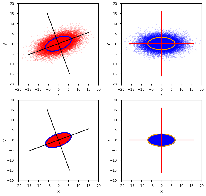
In the lower left corner we see a corresponding cut-off distribution Y_C – truncated at d_m = D. The right side of the plot shows the distribution and its truncated version after a transformation to the MVN’s MA-CCS, which has its coordinate axes aligned with the eigenvectors of the cov-matrix Cov_Y. Our problem can now be reformulated:

• How do we get an estimated covariance matrix Cov_Y for our BVN from the numerically determined cov-matrix Cov_C of the sample representing Y_C depicted in the lower left quadrant?

Underestimated values …

A simple numerical integration of the required covariance integrals over the data of the core region can be performed with the help of Numpy’s “cov()“-function. We then get the following numerical values for the cov-matrix Cov_C,num of the truncated sample (after some rounding of the decimals):

The element values are obviously far off the values of the elements of the original Cov_Y-matrix.

What do we get for the rotated distribution in the MA-CCS? The matrix Cov_Y,rot resulting from the transformation of Cov_Y into the MA-CCS should become diagonal there. For our example case a transformation of Cov_C via a rotation matrix for the given angle φ ≈ 20.3° indeed results in:

Numpy’s cov()-integration for the rotated truncated sample data instead gives the following values:

The attentive reader notices that in both cases a common and seemingly element-independent correction factor of around 2.41 would bring the matrix elements close to the original values. The question arises:

• What is the mathematical reason for this indication of an element-independent correction factor in our experiment? Can this finding be generalized and how can we calculate such a correction factor for different values of D and n?

Without any mathematical proof, the independence of the correction factor of the element could have occurred accidentally. Note: If you had done numerical experiments for other values of D, the resulting values of related correction factors would differ from the value given above – without showing a simple and clear dependence on D.

Are the 1-dimensional marginals of the cut-off distribution Gaussians?

Before we dive deeper, I want you to look at the projections of our cut-off example distribution onto the coordinate axes of the MA-CCS:

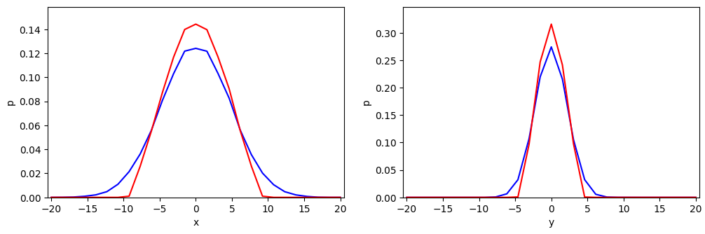
The graphs were derived by projections of the BVN sample onto the coordinate axes and by grossly sampling resulting data point numbers for equally sized intervals along the axes. Note that the resolution is limited due to the available number of data points in the sample and my choice of the interval size.

The red line shows the marginals along the x-axis (in the left plot) and along the y-axis (in the right plot). The blue lines show the respective marginals of the original infinite BVN. Both plots were normalized with respect to the available amount of data points inside the core (red lines) and to the total available number of points in the created sample (blue lines).

The differences between the shapes of the one-dimensional distributions result from the following fact:

• A projection of points of the infinite BVN onto the axes per unit length includes points coming from infinitely long stripes vertical to the axes. A projection of the cut-off distribution, instead, only includes corresponding points up to the elliptical border of the core area.

Note that we will have to deal with this problem also in the n-dimensional case, but then for a limiting (n-1)-dimensional ellipsoidal surface manifold and infinite columns over (n-1)-dim infinitesimal areas. This deviation from a MVN, of course, affects both theoretically derived as well as numerically determined values of the different cov-matrices.

A sense of intricate integrals …

The reader, of course, remembers that the elements of the covariance matrix of a multidimensional probability distribution are defined by volume integrals over the n-dim region covered by the distribution. The integrands are composed of products of two components of the position vectors r – multiplied with the probability density p(r) (per n-dim unit volume) at the position given by r. The components themselves can be derived by proper subsequent projections of the position vector onto coordinate planes and from there onto coordinate axes. These projection operations typically involve n angles (and related factors given by trigonometric functions) in n-dim polar coordinates. The projection results also depend on r = |r|. Just consider a 3-dim example.

Somewhere else in this blog, I have already and explicitly explicitly shown that the covariance matrix of BVN can indeed be derived from integrals over the (infinite) ℝ². However, I have not yet discussed a similar (explicit) integration of the corresponding terms for a general MVN covering the ℝⁿ. I will come back to this point in the next post – and we will learn something important from the respective integration procedure.

For a cut-off MVN the calculation of the elements of the covariance matrix must be performed up to a finite Mahalanobis distance. This indicates that the integration should be carried out for ellipsoidal shells of constant probability density given at constant Mahalanobis distances. Expressed in n-dim spherical coordinates we therefore await integrands of the volume integral of the following type:

with dσ(r_e) defining an angle dependent infinitesimal surface element at r_e – and r_e itself being bound to ellipsoidal surfaces.

At first sight, our mathematical intuition tells us that spherical coordinates may not be suited to solve this task in an easy way. You may, therefore, be tempted to integrate the products of the vector components over ellipsoidal surfaces first and afterward evaluate a remaining integral along the Mahalanobis distance as a kind of radial variable. This would require a transformation of the whole problem to elliptical coordinates and the application of a respective Jacobi determinant. Which may induce new problems. We will later see whether and how the transformation to n-dim elliptical coordinates can be circumvented.

Potentially working in ellipsoidal coordinates would be a somewhat unpleasant endeavor, already. But, while most of the resulting integrals can be solved for the infinite ℝⁿ, the situation gets much more complicated for the same integrals up to finite borders. Evaluating the surface integrals over ellipsoidal surfaces – or even surfaces of n-dimensional spheres (“balls”), if we are lucky – already poses a major problem, because these integrals involve a lot of multidimensional trigonometry. In addition, the remaining integral is of the type

Experienced readers already get an idea of the problems awaiting us. Other readers may need to search a while on the Internet for an explicit solution or may even be misguided by some stupid AI regarding steps for the achievement of a solution.

And as already indicated: Obstacles may result from the fact that the marginals of the geometrically cut-off distribution do not represent lower dimensional MVNs (or in the extreme case Gaussians along CCS-axes up to a coordinate values corresponding to d_m=D).

Conclusion

An infinite MVN distribution is well defined by its covariance matrix. However, a kind of reverse problem, namely the proper estimation of the elements of this matrix based on a sample of data points which reside inside some finite ellipsoidal core region of the MVN, appears to be an intricate problem. The task is related to the problem of mathematically determining the covariance matrix for a limited ellipsoidal core of a MVN. Such a core is defined by a finite Mahalanobis distance d_m=D. Outside the core the probability density is set to zero, i.e. the distribution is cut off outside the core.

The mathematical task of the calculation of the covariance matrix of such a cut-off MVN-distribution comes down to the evaluation of complicated volume and surface integrals over ellipsoidal areas in elliptical or polar coordinates. The integrands of the surface integrals will probably consist of terms involving trigonometrical expressions giving us projections of position vectors onto coordinate axes in n-dimensional polar or elliptical coordinates. Furthermore, exponential functions for the probability density of multidimensional MVNs let us expect further difficulties with remaining integrals along the Mahalanobis distance variable up to the core’s surface.

In the next post of this series we will look closer at the mathematical terms and expressions which cover our problem. This will give us a much better idea of the integrals we really have to solve – actually in spherical n-dimensional polar coordinates. But this will only temporarily give us a feeling of relief. Stay tuned ….