Orthogonal projections of multidimensional ellipsoids – I – points on the ellipsoid that give us the surface points of the projection

A reader of a parallel post-series on n-ellipsoids has asked me how I could know what the matrix for the quadratic form of the orthogonal projection of a (n-1) dimensional-ellipsoid onto a (n-1)-dimensional sub-space of the ℝⁿ looks like. I had stated in previous posts that we can directly derive the elements of the matrix describing projections of ellipsoids or the covariance matrix of a projected multivariate normal distribution from the matrix defining the original ellipsoid. However, I have not yet explained, why this claim is true. I will do so in this post-series.

Actually, the question of the reader is a very interesting one. As we will see, it must, however, be reformulated. Ellipsoids are closed, surface manifolds, but the orthogonal projection of an ellipsoidal surface gives you a volume in the lower-dimensional target space. So, actually, we have to discuss the relation of quadratic forms for the surface manifold in the original space om the one hand side and the surface of the projection in the sub-space on the other side. The other critical question is, why we can assume that the projections of ellipsoids have an ellipsoidal surface, at all.

A convincing answer to the reader’s question must, therefore, include proofs of the following two points:
I) The orthogonal projection of a (n-1)-dimensional ellipsoid to a q-dimensional sub-space of the Euclidean n-dimensional ℝⁿ has a (q-1)-dimensional ellipsoidal border-surface.
II) There is a clear and directly usable relation between the matrices mediating the quadratic form of the original ellipsoid and the quadratic form defining the surface of the ellipsoid’s projected image.

These are the topics of this mini-series. Unfortunately, in some literature on multidimensional ellipsoids, point (I) above is taken as granted. But the proof is not trivial. At least for people whose primary domain of knowledge is not math. So, an outline of the proof may be helpful for other readers, too. In this first post, I will discuss some geometrical arguments. After some math they will provide us with an insight that leads us to an elegant way of proving claim (I) for a projection onto a sub-space orthogonal to any given vector (topic of post II). In a third post we look at the relations of controlling matrices.

Relevance of orthogonal projections of ellipsoids for different application fields

The named problem, of course, also touches properties of Multivariate Normal Distributions [MVNs] and their projections to lower-dimensional sub-spaces. But, reversely, it also is relevant for the reconstruction of MVNs or ellipsoids from their projection images in low-dimensional spaces. This directly leads to the question how the variance-covariance matrices of a MVN and of its projections are related. The same for the question how we get the elements of matrices controlling the quadratic form of a high-dimensional ellipsoid from matrices controlling its projections.

In the numerical domains of statistics and Machine Learning, there is e.g. the question how we can reconstruct points inside the volume of a (n-1)-dimensional ellipsoid from their projected elliptical images in 2-dimensional coordinate planes and how the coordinates of points in one projection are related to the coordinates of the same points in another projection. The relation between projections of ellipsoids and the original ellipsoid is also a topic when analyzing MVN-like distributions or MVN-like cores with the help of the PCA-method.

The relation between projections of a multidimensional ellipsoids registered on multiple planes and the original ellipsoid itself is of general interest in physics and astrophysics, too. E.g. for experiments where data coming from an approximately ellipsoidal volume are registered in planes.

Geometrical aspects

To get to the aspired proofs, we will first look at some geometrical aspects of the projections of multidimensional ellipsoids. One such aspect is related to the question how we can describe, identify and create those special points on the original ellipsoidal surface which determine the border of the orthogonal projection of the ellipsoid. Readers of this blog know already that an ellipsoid can be created by a applying a linear transformation to vectors of a (n-1)-dimensional unit sphere. I.e., we want to identify points on the unit sphere which get transformed by a (n x n)-matrix A to image points on the ellipsoid whose tangential spaces control the projection. At the end of this post, we will use the result to explicitly identify such points by a numerical algorithm for ellipsoids in the ℝ³ below.

Suppositions and basic relations

We work in the (Euclidean) ℝⁿ. “dim” is used as an abbreviation of “dimensional”. CCS is an abbreviation for “Cartesian Coordinate System”. Unit vectors along the coordinate axes of the CCS covering the ℝⁿ are named e_i.

A centered ellipsoid is given by a set of points (vectors x_e,n) fulfilling

\[ E \,=\, \left\{ \pmb{x}_{e,n} \,\,\,| \,\,\, \pmb{x}_{e,n} = \pmb{\operatorname{A}} \pmb{u}_n \right\}, \quad \text{with} \,\,\, ||\pmb{u}_n|| = 1 \,. \tag{1} \]

A is an invertible matrix. The set of u_n-vectors define the (n-1)-dim unit-sphere 𝕊_n-1. By “centered” we mean that the center of the enclosed volume and the mean of all vectors coincides with the origin of the CCS, The quadratic form of the ellipsoid is given by a symmetric, invertible, positive-definite matrix Σ^-1

\[ \begin{align} &\pmb{\operatorname{\Sigma}}^{-1} \,=\, \left[ \pmb{\operatorname{A}} \pmb{\operatorname{A}}^T \right]^{-1} \,=\, \left[\pmb{\operatorname{A}}^T \right]^{-1} \, \pmb{\operatorname{A}}^{-1} \,, \tag{2} \\[10pt] & \pmb{x}_{e,n}^T \,\, \pmb{\operatorname{\Sigma}}^{-1} \, \pmb{x}_{e,n} \,=\, 1 \,. \tag{3} \end{align} \]

The reader recognizes these formulas from the discussion of MVNs and related confidence ellipsoids in this blog. Also Σ is symmetric, invertible and positive-definite. In the case of MVNs Σ represents the variance-covariance matrix.

Projections of closed surfaces give us lower-dimensional volumes

We just look at this important point with the help of an example. A basic insight, which is easy to prove, is that the image of the orthogonal projection of a unit-sphere onto a (n-1) dimensional sub-space (e.g. spanned by n-1 coordinate axes) is a (n-1)-dimensional unit ball and not a (n-2)-dimensional unit sphere. Just think about a projection of the points of the 2-dim surface of a unit-ball in the ℝ³ down to a 2-dim coordinate plane. I omit the rather simple proof.

This means that the (orthogonal) projection of a (n-1) dimensional ellipsoid will give us some (n-1) dimensional volume in a (n-1)-dim subspace. This means: To identify the form of the surface of the projection we will need to care about special points on the surface of an ellipsoid. Those points would mark a tangential space in the sense that the axis along which we project to an orthogonal subspace is orthogonal to the tangential space. Intuitively, we expect that the distance from the line of projection would be maximal at these points.

We start with discussing an ellipsoid in the ℝ³ and its tangent planes. This will help us to identify properties at points whose projection images are border points on the ellipsoid’s projection image. The derivation of claim (I) will be based on a central insight which the geometric approach leads us to.

Points on the ellipsoid which determine the border/surface of the projection

We use some wisdom of multidimensional calculus:

A: The gradient of a multidimensional function F(x₁, x₂, …,x_k, ..x_n) is perpendicular to its (n-1)-dimensional contour manifolds/surfaces at all points of such surfaces. This is an elementary result of calculus in Euclidean spaces, and I omit the proof.

Below we consider a projection along the direction of a selected coordinate axis and respective unit vector e_p onto the sub-space orthogonal to e_p. (In the next post we will generalize to other vectors.)

What can we say about those points which control the border of the ellipsoid’s projection image?

Guideline from the 3-dimensional geometry

Let our intuition for the 3-dim case help us. Let us use a CCS with x-, y– and z-axes. The z-axis looks upwards. The ellipsoids main axes are rotated against the coordinate axes. The projection of the ellipsoid shall happen along the y-axis onto the (x,z)-plane. I.e. e_p= e_y. We look at all points of the ellipsoid above the (x,y)-plane with z > 0. There is exactly one point in the (x,z)-plane for which z gets a maximum value. This point obviously is a member of the border of the projection’s image. Which point on the ellipsoid determines the projection with this maximum condition?

Move the (x,z) plane along the y-axis. Clearly, our critical point on the ellipsoid is one for which the z-coordinate takes a maximum value – depending on the varying x-, y-values. This means, we look for an extremum of z as a function of (x,y)-values, i.e. for an extremum of the function z(x,y).

The tangential plane at this special point has a normal vector parallel to the z-axis. This vector defining the tangential plane ist therefore orthogonal to the y-axis, which in turn defines the projection plane. Now, let us look at a different CCS, which has x– and z-axis rotated by an angle in the plane orthogonal to the y-axis. Then the same argument as above holds. Thus, we get all points of the border of the projection image by looking at those points on the ellipsoid whose tangent planes have a normal vector which is orthogonal to the projection direction given by e_y.

Try it out with an egg and a stiff paper sheet, but be careful with the egg … 🙂

Note that the gradient of a function F₃(x,y,z) which gives us our 3-dim ellipsoid as a contour surface is perpendicular to such a surface. I.e., we need to find points with the gradient of ∇F₃ ⊥ e_y.

The n-dimensional case

The argumentation in the general case is basically the same. You just have to replace the projection “plane” by projection “sub-space” and the tangent plane by a tangential subspace. We consider the direction of an e_k ⊥ e_p and its coordinate axis. The projection of points on the ellipsoid E into the sub-space with vectors orthogonal to e_p have varying x_k-values. We look at that part of the (n-1)-dim ellipsoid for which the x_k-values are positive. We interpret a coordinate value x_k as a function of all other coordinates x_k = x_k (x₁, …,x_k-1, _k+1, ..x_n). Again, the point on the ellipsoid determining a border point on the projection image P(E) with maximum x_k-value is given by an extremal value of x_k. Let us call the vector to such a “tangential” point (with respect to e_p) on the ellipsoid x^t_p,k ∈ E. Then we have

\[ \pmb{x} ^t_{p,k} \,:\, \quad {\partial \, x_k(x_1, ..x_{k-1}, x_{k+1}, …x_n) \over \partial \, x_i = 0} \,\, \text{with} \,\, i \ne k \,\, \land \, \, \pmb{x} ^t_{p,k} \in E \,. \tag{4} \]

The gradient of a function F_n (x₁, …x_n) which produces the ellipsoid as a contour surface should have a direction parallel to e_k and thus orthogonal to e_p. Why can we claim this in the multidimensional case?

Firstly, note that one can show that the second derivatives on the surface of an ellipsoid have the same sign in the surroundings of an extremum. You see this relatively easy in the main axes system. Also note that condition (3) regarding the quadratic form can be re-written as

\[ \sum_{i=1}^n \alpha_i \, x_i^2 \,+\, {1\over 2} \sum_{i,j \\ i \ne j}^n \beta_{i,j} \, x_i \, x_j \,=\, 1 \,, \quad \text{with}\,\, b_{i,j} = b_{j,i} \,, \tag{5} \]

with some constant coefficients α_i and β_i,j. Let us define a suitable function F_n which gives us concentric ellipsoids as contour surfaces:

\[ F(x_1, x_2, …, x_n) \,=\, \pmb{x}^T \, \pmb{\operatorname{\Sigma}}^{-1} \, \pmb{x} \,-\, 1 \,. \tag{6}\]

We could have used a density function of a MVN for this purpose. But that would have made things unnecessary complex. Our special ellipsoid is given by

\[ F(x_1, x_2, …, x_n) \,=\, 0 \,. \tag{7}\]

What is the gradient ∇F_n of F_n? We look at a specific partial derivative and take into account (5):

\[ {\partial F \over \partial x_i} \,=\, 2\alpha_i x_i + \sum^n_{j=1 \\ j \ne i} \, \beta_{i,j} \, x_j \,. \tag{7} \]

Note that from (7) one can not draw any direct conclusions regarding the gradient at such points. We need secondary information.

Regarding x_k = x_k(x₁, …,x_k-1, _k+1, ..x_n) we can combine (5) with the requirement that the partial derivatives of this function should be zero at our critical points. We again look at (5), but this time focusing on x_k().

\[ \begin{align} &\alpha_k \, x_k^2( x_1, ., x_i, …x_{k-1}, x_{k+1}, .. x_n) + \beta_{i,k} \, x_i \, x_k( … x_i,…x_n) \\[8pt] & =\, 1 \,-\, {\huge[} \sum^n_{m=1 \\ m \ne k} \, \alpha_m \, x_m^2 {\huge ]} \,-\, {\huge [}{1 \over 2} \, \sum_{l,m =1 \\ m \ne k}^n \, \beta_{l,m} \, x_l \, x_m {\huge]} \,. \tag{9} \end{align} \]

On a continuous ellipsoidal surface this function is two times differentiable. Note that the sums on the right side include the index “i“. Now, we apply a differentiation with respect to variable “x_i“:

\[ \begin{align} & 2 \, \alpha_k \,{ \partial \,x_k( x_1, ., x_i, …x_{k-1}, x_{k+1}, .. x_n) \over \partial \, x_i} + \beta_{i,k} \, x_k(…) + \beta_{i,k} \, x_i \, {\partial \, x_k(…) \over \partial \, x_i} \\[8pt] & – 2\, \alpha_i \, x_i \,-\, {\huge [}\sum_{m =1 \\ m \ne k}^n \, \beta_{i,m} \, x_m {\huge ]} \,. \tag{10} \end{align} \]

Now, we demand that the partial derivative on the left side gets zero. This leads us to:

\[ \begin{align} & \forall i \ne k \, : \quad 2\alpha_i x_i + \sum^n _{j=1, \\ j \ne i} \, \beta_{i,j} \, x_j \,= \, 0 \,, \tag{11} \\[10pt] & \Rightarrow \,\, {\partial \, F_n \over \partial \ x_i} \,=\, 0 \,, \quad \forall i \ne k \,, \tag{12} \\[10pt] & \Rightarrow \quad \nabla F_n \, \, || \,\, \pmb{e}_k \,\, \land \,\, \nabla F_n \perp \pmb{e}_p \,. \tag{13} \end{align} \]

(12) follows from the fact that the left side of (11) reflects a condition for all partial derivatives of F() with the exception of the variation in e_k-direction. I.e., an extremum of x_k on the surface is given at a point where the gradient is parallel to the coordinate axis e_k (- and where the Hesse matrix naturally fulfills the conditions of a maximum) (see 10 for 2nd order derivatives). The orthogonality with respect to e_p is a direct consequence.

Now our argument is valid for any direction of a unit-vector u_⊥p orthogonal to e_p : You just have to choose a different CCS with e_p kept fixed and with all other coordinate axes rotated around e_p , such that the rotated image of the original e_k coincides with u_⊥p . So for all of our critical points x_p^t on the surface determining the border of the orthogonal projection along e_p, we know

\[ \text{crit. tang. points on E} \,: \quad \nabla \ F_n(\pmb{x}^t_p) \bullet \pmb{e}_p \,=\, 0 \,. \tag{14} \]

\[ \]

Reconstruction of tangential points from points on the unit sphere

For practical purposes we would like to construct the critical tangential points on the ellipsoid from special points u_n^t of the unit sphere 𝕊_n-1 by applying the matrix A to these points (see eq. (1)). What can we say about these points on the unit sphere?

Due to the constant elements of the matrix Σ^-1 (see eq. (2)), the gradient of F_n can also be written in the following form:

\[ \nabla F_n (\pmb{x}) \,=\, 2 \, \pmb{\operatorname{\Sigma}}^{-1} \, \pmb{x} \,. \tag{15} \]

Condition (14) then is equivalent to

\[ \text{crit. tangent. points on E} \,: \quad \pmb{e}_p^T \, \pmb{\operatorname{\Sigma}}^{-1} \, \pmb{x}^t_p \,=\, 0 \,. \tag{16} \]

On the other side:

\[ \pmb{x}_p^t \,= \, \pmb{\operatorname{A}} \, \pmb{u}_n^t \,. \tag{17} \]

Taking into account eq. (2), this means

\[ \begin{align} & \pmb{e}_p^T \, \left[\pmb{\operatorname{A}}^T\right]^{-1} \, \pmb{\operatorname{A}}^{-1} \, \, \pmb{\operatorname{A}} \, \pmb{u}_n^t \,=\, 0 \,, \tag{18} \\[10pt] & \pmb{e}_p^T \, \left[\pmb{\operatorname{A}}^T\right]^{-1} \, \, \pmb{u}_n^t \,=\, 0 \,, \\[10pt] & \pmb{e}_p^T \, \left[\pmb{\operatorname{A}}^{-1}\right]^T \, \, \pmb{u}_n^t \,=\, 0 \,, \\[10pt] & \left[\pmb{\operatorname{A}}^{-1} \, \pmb{e}_p\, \right]^T \, \, \pmb{u}_n^t \,=\, 0 \,, \tag{19} \\[10pt] & \Rightarrow \quad \pmb{u}_n^t \, \perp \, \pmb{\operatorname{A}}^{-1} \, \pmb{e}_p\, . \tag{20} \end{align} \]

What does eqs. (1) and (20) tell us?All points on the unit sphere 𝕊_n-1, which fulfill eq. (19), must also reside in a subspace orthogonal to A^-1 e_p.

In a 3-dim space we would get these points as a cut of a plane orthogonal to A^-1 e_p with the unit sphere. So,

\[ \text{crit. tangent. points on E} \,: \quad \pmb{x}_p^t \,= \, \pmb{\operatorname{A}} \, \pmb{u}_n^t \,\, \land \,\, \pmb{u}_n^t \, \in \, \left\{ \pmb{u} \in \mathbb{S}^{n-1} \,\,|\,\, \pmb{u} \bullet (\pmb{\operatorname{A}}^{-1} \, \pmb{e}_p) \,=\, 0 \right\} \,. \tag{21} \]

This, actually, is a prescription of how to create such points on the ellipsoid.

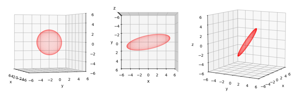
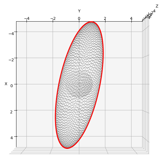
A example in three dimensions

The following plots show different perspectives of an ellipsoid with very different main axes in 3 dimensions. The quadratic form of the ellipsoid is given by a matrix Σ

\[ \pmb{\operatorname{\Sigma}} \, = \, \begin{pmatrix} \,\,21 & \,-4 & \,\,\, \, 6 \\ \,-4 & \,\,\,\, 3 &\,\,\, \, 2 \\ \,\,\,\,6 & \,\,\,\, 2 & \,\,\,\, 7 \end{pmatrix} \tag{22} \,. \]

You may take its inverse to get Σ^-1 . A Cholesky decomposition will give you a valid matrix A to construct the ellipsoid from vectors of unit sphere 𝕊₂.

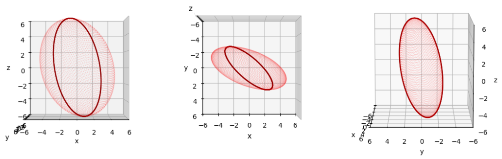
ellipsoid with very different main axes in 3-dim space

The following plot shows the points on the unit sphere which will give us the border points of the orthogonal projection onto the (y,z)-plane, i.e. e_p = e_x.

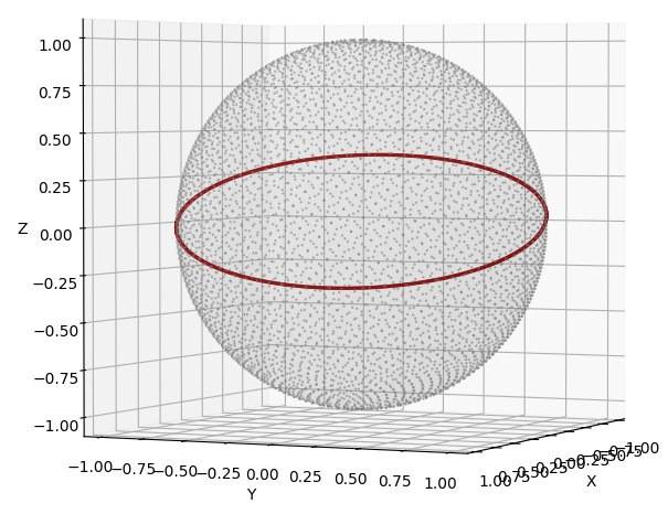
Hint: For those who want to perform the numerical experiment by themselves and are in doubt how to use (21) for defining a series of such points on the unit sphere 𝕊₂: You may use the cross vector product v = [(A^-1e_p) x e_z] of the vector A^-1 e_p and e_z to get a vector in the required plane. Normalize it to length 1. Then apply the cross-vector product once again between A^-1 e_p and v to get a second base vector in the plane. Afterward parameterize a unit circle in the plane. Then apply matrix A to get and plot the points on the ellipsoid.

Now, if everything is correct, we should exactly see the points after a transformation with A at the border of the ellipsoid when we look at the ellipsoid along the x-axis (azimuth=90; elevation=0). This is actually the case.

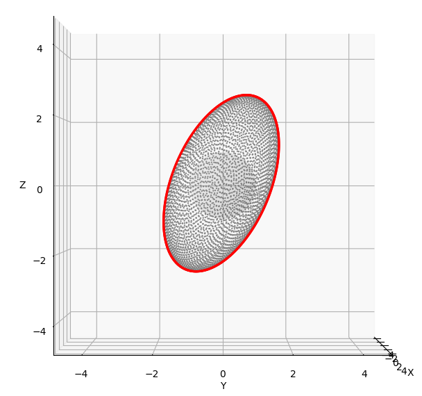
Points on ellipsoid giving the border-points of a projection onto the (x,z)-plane –
constructed via relation (21) and application of matrix A (e_p = e_x)

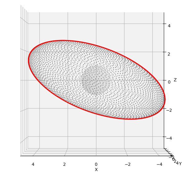
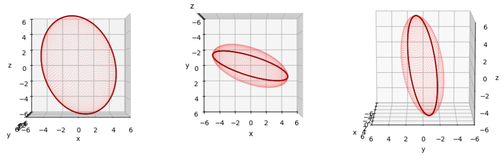
Below you see analogous results for the orthogonal projection onto the (x,z)-plane and the (x,y)-plane:

Points on ellipsoid giving the border-points of a projection onto the (y,z)-plane –
constructed via relation (21) and application of matrix A (e_p = e_y)

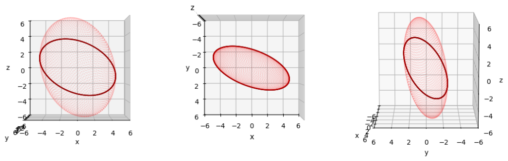
Points on ellipsoid giving the border-points of a projection onto the (y,z)-plane –
constructed via relation (21) and application of matrix A (e_p = e_z)

Readers who have repeated the experiment on their own may find the following: Due to the extreme form of the ellipsoid the calculated points are close to the border even when looked at the ellipsoid from different perspectives. Therefore, we need a different example.

Another example in three dimensions

Change the defining matrix to:

\[ \pmb{\operatorname{\Sigma}} \, = \, \begin{pmatrix} \,\,21 & \,\,\,\,6 & \,-5 \\ \,\,\,\,6 & \,\,\,\, 7 &\,\,\, \, 6 \\ \,-5 & \,\,\,\, 6 & \,\,36 \end{pmatrix} \tag{22} \,. \]

The following plots show the relevant points for different projections on the (y,z)-plane, the (x,z)-plane and the (x,y)-plane. Only from an appropriate perspective the calculated points mark the border of the points in the respective orthogonal projection.

Projection onto the (y,z)-plane

Projection onto the (x,z)-plane

Projection onto the (x,y)-plane

This gives us confidence in the whole mechanism.

What we still need to prove …

We know now which points on an ellipsoid’s surface give us the border points of the ellipsoid’s orthogonal projection image in a sub-space orthogonal to a coordinate axis (e_p) of a CCS covering the ℝⁿ. We still have to prove that the border-points of the projection follow a quadratic form and give us a (n-2)-dimensional ellipsoid. Only then we can investigate the connection between the matrices governing the quadratic forms of the original ellipsoid and the border of its orthogonal “shadow” in the target sub-space. These will be the subjects of further posts in this mini-series.

Conclusion

Orthogonal projections of multidimensional ellipsoids in the ℝⁿ onto (n-1) dimensional sub-spaces are of importance in statistics, physics and Machine Learning. An ellipsoid is given by the application of a matrix A upon vectors of the unit sphere 𝕊_n-1 and a resulting quadratic form. In this post we have regarded projections onto sub-spaces which were orthogonal to a unit vector e_p along the axis of a Cartesian coordinate system. We have derived how we can calculate the vectors for those points on the ellipsoid for which the projection results in the outmost border points of the ellipsoid’s projection image. We have found that the points on the ellipsoid can be constructed from points on a unit sphere, which are given by a cut with a sub-space orthogonal to a special vector A^-1 e_p. In the next post, we will use this insight to prove that the border surface in the projection sub-space forms a (n-2)-dimensional ellipsoid.