n-dimensional spheres and ellipsoids – IV – numerical check of Rivin’s formula for the surface areas of ellipsoids in 3 dimensions and the perimeters of ellipses

In the third post of this series we have discussed an idea of I. Rivin (see [1], [2]). Rivin has shown that the surface area of a general (n-1)-dimensional ellipsoid in a n-dimensional Euclidean space can be expressed in terms of an expectation value of a specific function weighted by a multivariate Gaussian probability density [pdf]. In contrast to (n-1)-spheres and n-balls, the ratio between the surface area of a (n-1)-ellipsoid and its enclosed n-dimensional volume is given by a complicated expression.

One can show that already the determination of the surface area of a 2-dimensional ellipsoid in the ℝ³ requires the (numerical) evaluation of complete and incomplete elliptic integrals; see [9] for details. For n-ellipsoids one must either evaluate a Lauricella hypergeometric function (series) [10] or Abelian integrals [11]. Rivin’s formula instead allows for a numerical calculation of the surface of (n-1)-dimensional ellipsoids by averaging data of a specific function multiplied with the pdf of a standardized Multivariate Normal distribution [MVN]. This finding links statistics and geometry in an exciting way.

In this post we will show that Rivin’s ideas really work. At least for low-dimensional ellipsoids. For ellipses and ellipsoids in the ℝ³ very good approximation formulas are available; see e.g. a discussion by J.D. Cook in [3] and [4]. We will use these approximations below in numerical experiments and compare their results to Rivin’s expectation values for ellipses and ellipsoids in a 3-dimensional space. We will find a very good agreement.

Previous posts in this series:

Reminder – Rivin’s formula

We define a (n-1)-dim ellipsoid with semi-axes a_i (i ∈ [1,n] ) in the (Euclidean) ℝⁿby

\[ \begin{align} & E \,=\, \left\{ x \in \mathbb{R}^n \,\,\,\,|\,\,\,\, \sum_{i=1}^n \, q_i^2 \ x_i^2 = 1 \, \right\}\,, \tag{1} \\[10pt] & \text{with} \,\, q_i := {1 \over a_i} \,. \tag{2} \end{align} \]

Note: This description implies a special choice of a Cartesian Coordinate System [CCS], namely one whose coordinate axes are aligned with the ellipsoid’s n main axes. In addition, the ellipsoid’s geometrical center must coincide with the CCS’ origin.

The “(n-1)” refers to the dimensionality of the ellipsoidal manifold. Rivin claims in [1], [2]:

\[ S_{n-1}(E) \,=\, 2 \, \pi^{n/2} \, { 1 \over \Gamma \left( {n+1 \over 2 }\right) } \, \left[\prod_{i=1}^n \, a_i \right] \, \, \mathbb{E} \left( \sqrt{ q_1^2 \, X_1^2 + q_2^2\, X_2^2 + \, … + q_n^2 \, X^2_n \, } \, \right) \,, \tag{3} \]

where the expectation value is given by

\[ \begin{align} & \mathbb{E} \left( \sqrt{ q_1^2 \, X_1^2 + q_2^2\, X_2^2 + \, … + q_n^2 \, X^2_n \, } \, \right) \, = \, \\[10pt] &\quad \, { 1 \over \sqrt{2} } \, \, \int_{\mathbb{R}^{n}} \, { 1 \over (2\pi)^{n/2} \, } \, \exp \left(- \, {1\over 2} \, v^2\right) \, \, \sqrt{ q_1^2 \, v_1^2 + q_2^2\, v_2^2 + \, … + \, q_n^2 \, v^2_n \,\, } \,\, dv_1\, dv_2\, …\ dv_n \,. \tag{4} \end{align} \]

This means that we have to average the square root for a probability density of n independent Gaussians of a very elementary standardized and thus radially symmetric MVN (covering all of the ℝⁿ).

How can we check the formula numerically for ellipsoids and ellipses in the ℝ³?

Below we will use a 4-dim MVN to first create four different 3-dimensional MVNs [3D-MVNs]. Afterwards, we describe the statistically generated vectors of each 3D-MVN in the main-axes system of the MVN’s concentric contour ellipsoids. A standardization of the resulting distribution of data points and respective vectors eventually allows for a numerical calculation of Rivin’s expectation value for any confidence ellipsoid defined by a distinct value of a Mahalanobis distance. For ellipsoids and ellipses, there exist very good approximation regarding the surface area and the perimeter, respectively.

Exact formulas for the perimeter of an ellipse and the surface area of an ellipsoid in a 3-dim space

We find the exact formula for the perimeter of an ellipse S_1,ell in terms of a complete elliptic integral E_c in [6]:

Perimeter of an ellipse

\[ S_{1,ell} \,= \, 4 \, a \, E_c(e^2), \quad \text{with} \,\,\, e \,=\, \sqrt{ 1 \,-\, {b^2 \over a^2}\, } , \quad a \ge b \,. \tag{5} \]

E_c(e) represents the complete elliptic integral of the second kind. e is the ellipticity of the ellipse. The SciPy library provides functions to calculate E_c with a high degree of accuracy.

C. Hill gives an exact formula for the surface of a 2-dimensional ellipsoid in the ℝ³ in terms of incomplete elliptic integral of the first and second kind (see [9]):

Surface of an ellipsoid in the ℝ³

\[ \begin{align} & S_{2,ell} \,= \, 2 \pi \, c^2 \, +\, {2\,\pi\, a\, b \over \sin \phi } \, \left( K(\phi, k^2 ) \, \cos ^2 \phi \,+\, E(\phi, k^2) \,\sin^2\phi \right) \,, \\[10pt] & \text{with} \quad \cos \phi \,=\, {c \over a }, \quad k \,=\, { a \over b } \, { \sqrt{ b^2 \,-\, c^2} \over \sqrt{a^2 \,-\, c^2} }, \quad a \ge b \ge c \,. \end{align} \tag{6} \]

In this formula a, b, c represent the semi-axes, with a being the largest and c the smallest semi-axis (!). So, to apply the formula you first have to order the semi-axes. K(Φ,k) and E(Φ,k) represent incomplete elliptic integrals of the first and second kinds, respectively. The SciPy library provides functions to calculate these integrals with a high degree of accuracy.

Below, we will take the above formulas (in their SciPy approximation) as the standard values with which we compare the results of numerical evaluations of Rivin’s formula.

Approximation formulas for the surface areas of ellipsoids and ellipses

A physicist, J.D. Cook, has written about approximation formulas for the surface areas of ellipsoids in 2 and 3 dimensions (see [3] and [4]). For an ellipse with semi-axes a and b Cook cites the following approximation of Linderholm and Segal [5]:

Approximation 1 for the perimeter of an ellipse

\[ S_{1,ell} \,\approx \, 2 \pi \, \left( {a^{3/2} + b^{3/2} \over 2}\,\right)^{2/3} \,. \tag{7} \]

We find another approximation of Ramanujan at Wikipedia [6]:

Approximation 2 for the perimeter of an ellipse

\[ S_{1,ell} \,\approx \, \pi \,( a+b) \left( 1 + {3\,h \over 10 + \sqrt{4 – 3h \, } } \right) \,, \,\,\,\, h \,=\, { (a -b)^2 \over (a+b)^2 } \,. \tag{8} \]

For a 3-dimensional ellipsoid with semi-axes a, b, c, J.D. Cook [4] and also G.P. Michon [7] name a formula given by Knud Thomsen (2004, see [7] ). You find this formula also on Wikipedia [8]:

Approximation for the surface of a 3D-ellipsoid

\[ S_{2,ell} \,\approx \, 4 \pi \, \left( { (a\,b)^p + (b\,c)^p + (a\,c)^p \over 3} \right)^{1/p} \,, \,\,\,\, p \,=\, 1.6075 \,. \tag{9} \]

Another approximation is discussed by C. Hill in [9]

\[ \begin{align} &S_{2,ell} \,\approx \,2 \pi \, c^2 \, +\, 2\pi a b r \, \left( 1\,-\, r^2\, \, {b^2 – c^2 \over 6\, b^2 } \left( 1 \,-\, r^2 \, {3 b^2 + 10 c^2 \over 56\, b^2 } \right) \right) \,, \\[10pt] & \text{with} \,\,\, r \,=\, {\phi \over \sin\phi} \,. \end{align} \tag{10} \]

So, we have a variety of approximations to choose from.

Setup of the numerical experiment

Below, we call the main-axes CCS of a MVN’s contour ellipsoids the “MVN’s main-axes system”. To test Rivin’s formula we use the following setup and steps:

Step 1: We use a (4×4)-covariance matrix to create a 4-dimensional MVN in the (Euclidan) ℝ⁴ . The main axes of this 4D-MVN’s ellipsoids are rotated against the CCS’ coordinate axes. The creation of respective data points is done with the help of Numpy’s function random.multivariate_normal().
Step 2: We project the 4-dim MVN down to 4 different 3-dimensional ℝ³ sub-spaces of the ℝ⁴. The projection is done to sub-spaces orthogonal to the 4 coordinate axes. These projections give us four 3-dimensional 3D-MVNs. The axes of their contour ellipses are rotated against the coordinate axes of the 3-dim sub-space.
Step 3: For the 3-dim MVNs we can get their (3×3)-covariance matrices [cov-matrices] by selecting related elements out of the original (4×4) matrix. The selection corresponds to the application of a projection matrix.
Step 4: From the eigenvalues of the (3×3) cov-matrices we can evaluate the semi-axes of related contour ellipsoids or confidence ellipses given by some Mahalanobis distances d_m.
Step 5: From the eigenvectors of each (3×3) cov-matrix we get the rotation matrix required to describe the vectors of the 3-dim MVN in the MVN’s main-axes system. (The coordinate axes of the respective CCS for the 3-dim sub-space are then aligned with the main axes of the concentric contour ellipsoids.) We transform all the vectors given for the generated data points of each 3-dim MVN into the its main-axes CCS. We also use the rotation matrix to transform each 3D-MVN’s covariance matrix into its main-axes coordinate system. This corresponds to a diagonalization.
Step 6: We standardize the four 3-dim MVNs in their main-axes system and get respective spherically symmetric MVNs of decoupled independent Gaussians. As we are already in the main axes system of each of the 3D-MVNs, this operation corresponds to simple divisions of the coordinate values by a respective eigenvalue of the transformed cov-matrix.
Step 7: Step 6 allows for the calculation of the required evaluation value in Rivin’s formula, which we compare with results of independent (approximation) formulas (6), (9) and (10).

Note: The change to the main-axes system of each 3D-MVN in step 5 is an essential operation. Note further that during step 7 the numerical averaging is done via the number of data points.

Afterward we do something analogously with projections on 2-dim sub-spaces of the ℝ⁴. This then gives us 6 different 2-dim MVNs, which we use to test Rivin’s formula for the perimeters of respective confidence ellipses. We compare the results to formulas (5), (7) and (8).

As a starting point for step 1, we use the following (4×4)-cov-matrix:

\[ \operatorname{cov} \, = \, \begin{pmatrix} \,\,21 & -4 & \,\,\,\, 6 & -5 \\ -4 & \,\,\,\, 3 & \,\,\,\, 2 & \,\,\,\, 5 \\ \,\,\,\,7 & \,\,\,\, 2 & \,\,\,\, 7 &\,\,\, \, 6 \\ -5 & \,\,\,\, 5 & \,\,\,\, 5 & \,\,\, 36 \end{pmatrix} \tag{11} \,. \]

The 4-dim MVN is constructed with the help of Numpy’s function random.multivariate_normal(). We create 40,000 data points and respective vectors. The projections leave the number of points unaffected.

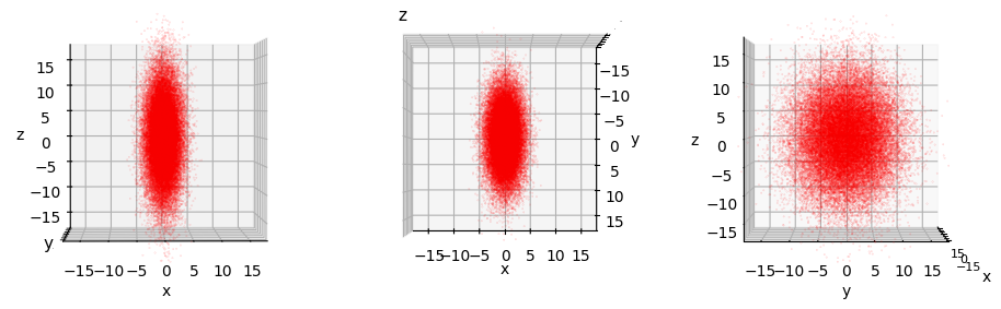
Plots and results for the surface areas of 4 ellipsoids

Below you find the 3-dim projections. Each line shows one of the four 3D-MVDs from 3 different perspectives. The 4 coordinate axes of the 4-dim space were named x0, x1, x2 and x3.

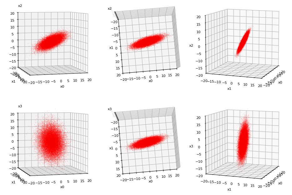
The real character and the differences between MVNs and the orientations of their main axes will become clearer after a representation in their main axes systems; see below.

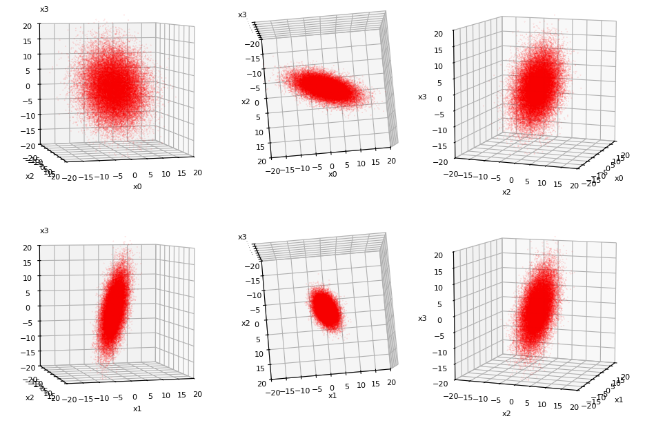
Main axes representations

In the same order as above the rotated 3-dimensional projection MVDs look like follows in their main-axes systems. Note that the axes have been renamed and the order of axes may be switched.

3-dim MVN 1:

3-dim MVN 2:

3-dim MVN 3:

3-dim MVN 4:

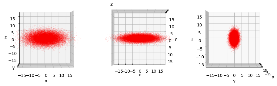
So, we really have 4 rather different ellipsoids shapes.

Note about the order of projection and rotation:
We have first projected the original 4-dimensional MVN and then rotated each 3-dimensional projection into the 3D-MVN’s main-axes system. For some tests this order has to be considered carefully during programming.

Table with results

The results in the following table depend a bit on the random generation and placement of the 4D-MVD’s data points. So two different runs may differ somewhat regarding relative deviations between the results. I started the generation of the 4D-MVD again ahead of calculating the data for another 3D projection MVN-x. The tables have the same order as the images of the 3-dim MVNs depicted above.

Concrete ellipsoids of the 3D MVNs were defined by distinct values d_m = 0.5, 0.75, 1.00, 1.25, 1.5, 1.75, 2.00 of the Mahalanobis distance d_m.

3-dim MVN 1:

3D-MVN	Formula	dm=0.50	dm=0.75	dm=1.00	dm=1.25	dm=1.50	dm=1.75	dm=2.00
3D-MVN 1	Surface exact eq.(6)	21.50625	48.38907	86.02502	134.41409	193.55629	263.45162	344.10007
3D-MVN 1	Surface acc. Rivin eq.(3)	21.47386	48.31619	85.89545	134.21164	193.26476	263.05481	343.58179
3D-MVN 1	Surface approx1 eq.(9)	21.68567	48.79276	86.74268	135.53543	195.17102	265.64944	346.97070
3D-MVN 1	Surface approx2 eq.(10)	21.24251	47.79565	84.97005	132.76570	191.18261	260.22077	339.88019

3-dim MVN 2:

3D-MVN	Formula	dm=0.50	dm=0.75	dm=1.00	dm=1.25	dm=1.50	dm=1.75	dm=2.00
3D-MVN 2	Surface exact eq.(6)	49.27788	110.87523	197.11151	307.98674	443.50090	603.65401	788.44605
3D-MVN 2	Surface acc. Rivin eq.(3)	49.36350	111.06789	197.45402	308.52190	444.27155	604.70294	789.81608
3D-MVN 2	Surface approx1 eq.(9)	49.55488	111.49848	198.21952	309.71799	445.99391	607.04727	792.87806
3D-MVN 2	Surface approx2 eq.(10)	47.55979	107.00952	190.23915	297.24867	428.03808	582.60739	760.95659

3-dim MVN 3:

3D-MVN	Formula	dm=0.50	dm=0.75	dm=1.00	dm=1.25	dm=1.50	dm=1.75	dm=2.00
3D-MVN 3	Surface exact eq.(6)	55.74462	125.42540	222.97848	348.40388	501.70159	682.87161	891.91394
3D-MVN 3	Surface acc. Rivin eq.(3)	55.77960	125.50410	223.11840	348.62249	502.01639	683.30009	892.47358
3D-MVN 3	Surface approx1 eq.(9)	55.95887	125.90746	223.83549	349.74295	503.62985	685.49619	895.34196
3D-MVN 3	Surface approx2 eq.(10)	53.07174	119.41142	212.28697	331.69838	477.64567	650.12883	849.14786

3-dim MVN 4:

3D-MVN	Formula	dm=0.50	dm=0.75	dm=1.00	dm=1.25	dm=1.50	dm=1.75	dm=2.00
3D-MVN 4	Surface exact eq.(6)	30.89089	69.50451	123.56358	193.06810	278.01806	378.41347	494.25433
3D-MVN 4	Surface acc. Rivin eq.(3)	30.89478	69.51326	123.57914	193.09240	278.05305	378.46110	494.31654
3D-MVN 4	Surface approx1 eq.(9)	30.88839	69.49889	123.55358	193.05246	277.99554	378.38283	494.21430
3D-MVN 4	Surface approx2 eq.(10)	30.34089	68.26701	121.36357	189.63058	273.06803	371.67593	485.45428

The numerical evaluation of Rivin’s formula obviously delivers excellent results. The relative error err_rel in comparison to eq. (6) is around or smaller than err_rel ≈< 0.002.
The 1st approximation acc. to eq. (9) also works very well. However, the second approximation acc. to eq. (10) comes with somewhat bigger relative errors in the range of some percent.

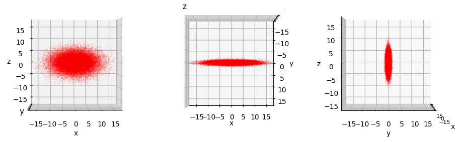
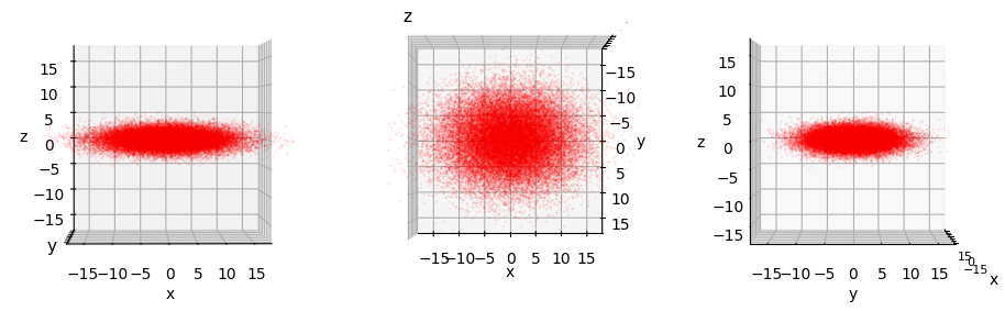
Results for 2-dimensional projections and the perimeters of respective ellipses

We now look at the six 2-dimensional projections onto coordinate planes and calculate the ellipses’ perimeters with the help of Rivin’s formula. The 2-dim projections are shown in the following illustration:

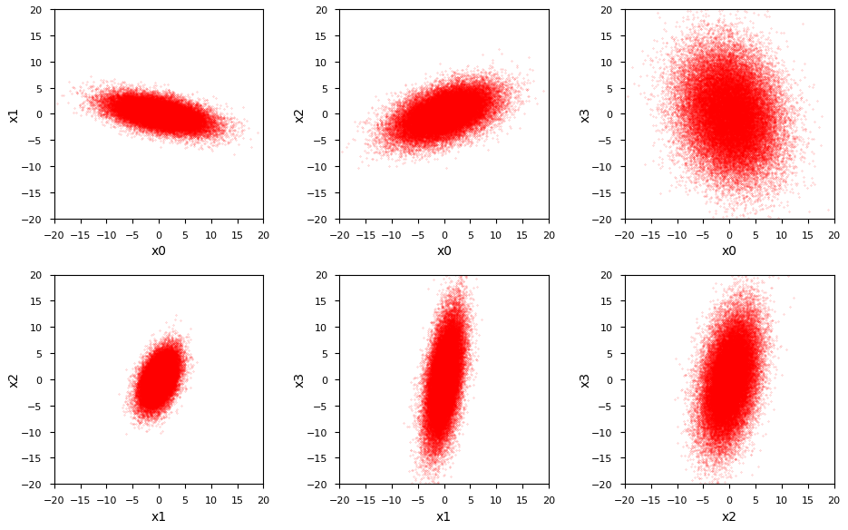
I omit images displaying the distributions in themain-axes systems of the respective contour ellipses of these six 2-dim distributions.

Concrete Contour ellipses are again defined via different Mahalanobis distances d_m.

2-dim MVN 1:

2D-MVN	Formula	dm=0.50	dm=0.75	dm=1.00	dm=1.25	dm=1.50	dm=1.75	dm=2.00
2D-MVN 1	Surface exact eq.(5)	10.31620	15.47430	20.63240	25.79051	30.94860	36.10671	41.26481
2D-MVN 1	Surface acc. Rivin eq.(3)	10.30272	15.45407	20.60543	25.75679	30.90815	36.05951	41.21086
2D-MVN 1	Surface approx1 eq.(7)	10.30523	15.45784	20.61046	25.76308	30.91569	36.06831	41.22092
2D-MVN 1	Surface approx2 eq.(8)	10.31620	15.47430	20.63240	25.79050	30.94861	36.10671	41.26481

2-dim MVN 2:

2D-MVN	Formula	dm=0.50	dm=0.75	dm=1.00	dm=1.25	dm=1.50	dm=1.75	dm=2.00
2D-MVN 2	Surface exact eq.(5)	11.39554	17.09334	22.79109	28.48886	34.18663	39.88440	45.58218
2D-MVN 2	Surface acc. Rivin eq.(3)	11.38664	17.07996	22.77328	28.46659	34.15991	39.85323	45.54655
2D-MVN 2	Surface approx1 eq.(7)	11.39216	17.08823	22.78431	28.48039	34.17647	39.872546	45.56862
2D-MVN 2	Surface approx2 eq.(8)	11.39554	17.09332	22.79109	28.48886	34.18663	39.88440	45.58218

2-dim MVN 3:

2D-MVN	Formula	dm=0.50	dm=0.75	dm=1.00	dm=1.25	dm=1.50	dm=1.75	dm=2.00
MVN_3	Surface exact eq.(5)	16.66409	24.99613	33.32818	41.66022	49.99227	58.32431	66.65636
2D-MVN 3	Surface acc. Rivin eq.(3)	16.61967	24.92950	33.23934	41.54917	49.85900	58.16884	66.47867
2D-MVN 3	Surface approx1 eq.(7)	16.66391	24.99586	33.32782	41.65977	49.99173	58.32368	66.65564
2D-MVN 3	Surface approx2 eq.(8)	16.66409	24.99613	33.32818	41.66022	49.99227	58.32431	66.65636

2-dim MVN 4:

2D-MVN	Formula	dm=0.50	dm=0.75	dm=1.00	dm=1.25	dm=1.50	dm=1.75	dm=2.00
2D-MVN 4	Surface exact eq.(5)	6.87197	10.30796	13.74395	17.17993	20.61592	24.05191	27.48789
2D-MVN 4	Surface acc. Rivin eq.(3)	6.83515	10.25272	13.67029	17.08787	20.50544	23.92302	27.34059
2D-MVN 4	Surface approx1 eq.(7)	6.87101	10.30652	13.74202	17.17753	20.61304	24.04854	27.48405
2D-MVN 4	Surface approx2 eq.(8)	6.87197	10.30796	13.74395	17.17993	20.61592	24.05191	27.48789

2-dim MVN 5:

2D-MVN	Formula	dm=0.50	dm=0.75	dm=1.00	dm=1.25	dm=1.50	dm=1.75	dm=2.00
2D-MVN 5	Surface exact eq.(6)	12.98802	19.48203	25.97604	32.47005	38.96407	45.45808	51.95209
2D-MVN 5	Surface acc. Rivin eq.(3)	12.87278	19.30917	25.74556	32.18195	38.61834	45.05473	51.49112
2D-MVN 5	Surface approx1 eq.(9)	12.96426	19.44638	25.92851	32.41064	38.89277	45.37489	51.85702
2D-MVN 5	Surface approx2 eq.(10)	12.98802	19.48203	25.97604	32.47005	38.96407	45.45806	51.95207

2-dim MVN 6:

2D-MVN	Formula	dm=0.50	dm=0.75	dm=1.00	dm=1.25	dm=1.50	dm=1.75	dm=2.00
2D-MVN 6	Surface exact eq.(5)	14.00078	21.00118	28.00157	35.00196	42.00235	49.00274	56.00314
2D-MVN 6	Surface acc. Rivin eq.(3)	14.04203	21.06305	28.08407	35.10508	42.12610	49.14712	56.16813
2D-MVN 6	Surface approx1 eq.(7)	13.99352	20.99028	27.98704	34.98380	41.98056	48.97732	55.97408
2D-MVN 6	Surface approx2 eq.(8)	14.00078	21.00118	28.00157	35.00196	42.00235	49.00274	56.00314

What we see here is that Rivin’s formula is still very good: The relative errors err_rel under our conditions are in the range of err_rel ≈< 0.0055 and smaller.

However, the approximation formulas of Linderholm/Segal (7) and especially of Ramanujan (8) give you better results than our statistical numerical estimation.

Accuracy and number of statistical data points

An interesting question is how the accuracy varies with the number of data points. The problem is that with growing dimension the space we have to fill grows substantially. A first guess is that we need a certain number of data points per dimension to get a reasonable accuracy. In our case we would need 6 to 7 million points if we went to n=500. Which is many! So, let us go down to 800 points per dimension. That would mean 400.000 data points for n=500. (Such numbers are relatively common in modern Machine Learning.)

The following table shows that the relative error goes up to some percent due to the lower resolution of the MVN. The table contains values of the relative error of the evaluation of Rivin’s formula compared with values of eq. (6) for ellipsoids and eq. (5) for ellipses, evaluated for only two values of the Mahalanobis distance d_m = 0.5, 2.00. The order of the the MVNs corresponds to the order given above.

2D/3D	axes	dm=0.50	dm=2.00
3D	(0, 1, 2)	0.010	0.009
3D	(0, 1, 3)	0.015	0.025
3D	(0, 2, 3)	0.021	0.019
3D	(1, 2, 3)	0.017	0.017
2D	(0, 1)	0.024	0.024
2D	(0, 2)	0.021	0.022
2D	(0, 3)	0.015	0.014
2D	(1, 2)	0.015	0.018
2D	(1, 3)	0.029	0.028
2D	(2, 3)	0.011	0.012

The relative error is now around err_rel ≈< 0.03 – which is not very surprising. This is still a good value. It is an indication that between 500 to 1000 data points per dimension are sufficient to calculate the surface are of (n-1) dimensional ellipsoid with a relative error of some percent.

Conclusion

In this post we have used numerical means to show that Rivin’s formula based on MVN statistics indeed provides a correct value for the surface area of 2-dimensional ellipsoids in the ℝ³ and ellipses in the ℝ². Of course, using discrete data points in our evaluation came with relative errors. But the accuracy for our numerical settings was quite convincing. This strengthens our trust in Rivin’s formua for the evaluation of the surface area of n-ellipsoids. Note however that our tests can not replace numerical evaluations for a higher number of dimensions. I will discuss this point briefly in a forthcoming post.

Links and literature

[1] I. Rivin, 2003, “Surface Area of Ellipsoids”, DOI: 10.48550/arXiv.math/0306387,
https://arxiv.org/abs/math/0306387v4

[2] I. Rivin, 2004, “Surface Area And Other Measures Of Ellipsoids”, DOI: https://doi.org/10.48550/arXiv.math/0403375,
https://arxiv.org/abs/math/0403375

[3] J.D. Cook, 2021, “Simple approximation for surface area of an ellipsoid”, blog post at
https://www.johndcook.com/blog/2021/03/24/surface-area-ellipsoid/

[4] J.D. Cook, 2023, “Hyperellipsoid surface area”, blog post at
https://www.johndcook.com/blog/2023/09/11/hyperellipsoid-surface-area/

[5] C. E. Linderholm, A. C. Segal, 1995, “An Overlooked Series for the Elliptic
Perimeter”, Mathematics Magazine, June 1995, pp. 216-220

[6] Wikipedia article on “Perimeter of an ellipse”,
https://en.wikipedia.org/wiki/Perimeter_of_an_ellipse

[7] G. P. Michon, 2004, “Spheroids & Scalene Ellipsoids”,
https://www.numericana.com/answer/ellipsoid.htm#spheroid

[8] Wikipedia article on “Ellipsoid”,
https://en.wikipedia.org/wiki/Ellipsoid

[9] C. Hill, 2020, “Learning Scientific Programming with Python”, Cambridge University Press, https://doi.org/10.1017/97811087780391.
Online excerpt regarding approximations to elliptic integrals and the surface of an ellipsoid at
https://scipython.com/books/book2/chapter-8-scipy/problems/the-surface-area-of-an-ellipsoid/

[10] Paul Masson, Independent Physicist, San Francisco, 2021, contribution at analyticphysics.com on n-dimensional ellipsoids
https://analyticphysics.com/Higher%20Dimensions/Ellipsoids%20in%20Higher%20Dimensions.htm

[11] G. J. Tee, 2004/2005, “Surface Area And Capacity Of Ellipsoids In n Dimensions”, Department of Mathematics, University of Auckland, New Zealand,
https://www.math.auckland.ac.nz/deptdb/dept_reports/539.pdf
https://researchspace.auckland.ac.nz/server/api/core/bitstreams/64845042-d15c-4667-9ffe-c59682665f1d/content