Covariance matrix of a cut-off Multivariate Normal Distribution – III – results for a 2-dimensional BVN-core and proper normalization of its cut-off distribution

In the math section of this blog, we try to cover interesting aspects of Multivariate Normal Distributions [MVNs]. The topic of this post series is the covariance matrix of a MVN-like distribution confined inside a hyper-surface of constant probability density. Outside of the surface we set the probability density to zero. This gives us a “cut-off” MVN- distribution. Contour surfaces of a MVN in general enclose a central ellipsoidal volume in the MVN’s n-dimensional space. We have called such a volume a core.

We want to answer the following question: How does the covariance matrices of such a core and its cut-off MVN differ from the covariance matrix of the related standard MVN which stretches out to infinite distances in the n-dimensional space? In this post we are going to analyze the 2-dimensional problem for a cut-off Bivariate Normal Distribution [BVN] in detail. We will then use a respective sample of data points inside a finite Mahalanobis distance D to numerically test and verify theoretical predictions.

In a first step we will apply the results of the 2nd post in this series and evaluate required integrals in polar coordinates. The analytical result will confirm that the covariance matrix of the original MVN can be calculated by multiplying the core’s covariance matrix by a factor which is the same for all matrix elements. The core’s cov-matrix can be estimated from a numerical integration of respective sample data. We will, however, learn that we must apply an additional correction factor to compensate for a systematic difference still existing between our theoretical results and numerical integrations. This factor is given by a proper normalization of the cut-off distribution.

We use abbreviations and conventions defined in the 1st post of this series. Note that some authors use the abbreviations BVD, MVD instead of our acronyms BVN, MVN, respectively.

Previous posts

A two dimensional scenario

We reuse the 2-dim BVN-example already presented in the 1st post of this series. It was based on the following (2×2)-cov-matrix Σ₂ :

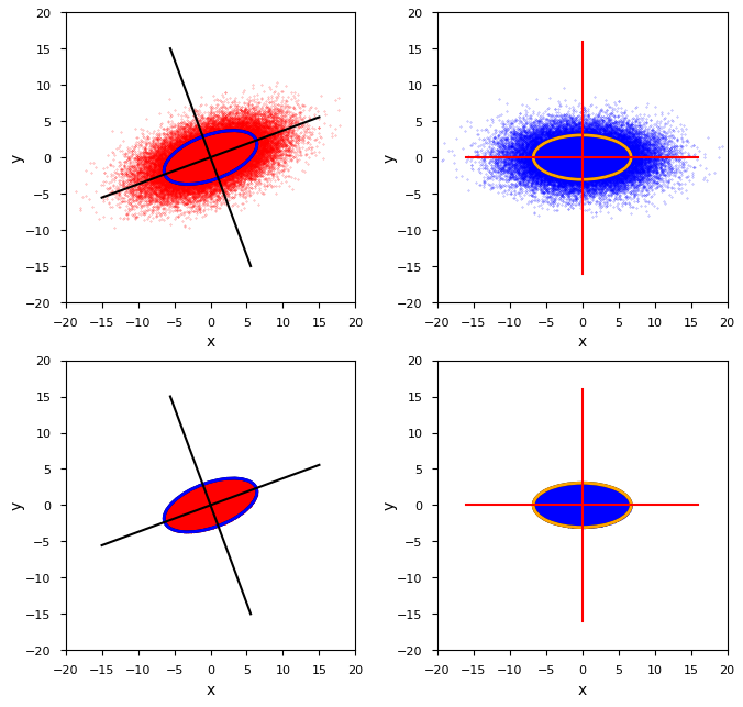
\[ \pmb{\operatorname{{Cov}_{2,Y}}} \,=\, \pmb{\operatorname{\Sigma}}_{2} \,=\, \begin{pmatrix} 21 & 6 \\ 6 & 7 \end{pmatrix} \,. \tag{1}\]

Cut-off BVN limited to an ellipsoidal core

We want to calculate the cov-matrix of the infinite distribution depicted in the upper left quadrant. The data available are, however, only data for the cut-off distribution depicted in the lower left corner. The value of the Mahalanobis distance d_m defining the surface of the core is

\[ d_m\, =\, D \,=\, 1.4 \,. \]

Let us in a first step analyze the situation mathematically for a general D. We, of course, use results of post 2.

Integrals to solve for the n-dim case

The random vector Y_N of a MVN has a probability density g(y) controlled by a symmetric and invertible covariance matrix Σ_Y = Cov_Y; see post 2. This density g(y) has contour surfaces surrounding the volume of an ellipsoid in the n-dimensional space of the MVN. In post 2, we have shown that we can nevertheless evaluate a volume integral over a spherical volume to get the covariance matrix Cov_C of the contents of a MVN’s ellipsoidal core:

\[ \pmb{\operatorname{Cov_C}} \,=\, \pmb{\operatorname{M}}_Y \left[ {1\over (2\,\pi)^{n/2} } \, \underset{ V_{n,D}^{sph}}{\iint …\int} \, \pmb{Z} \pmb{Z}^T \, \operatorname{exp} \left( -\, {1\over 2} \, \pmb{Z}^T \, \pmb{Z} \,\right) \, dz_1\,dz_2 \, ….\, dz_n \right] \pmb{\operatorname{M}}_Y^T \,. \tag{2} \]

The spherical volume is just a mapping of the original ellipsoidal core of Y mediated by the coordinate transformation [M_Y]^-1 that maps a general Y_N to Z. Z is the random vector of a special MVN-distribution build from independent 1-dimensional Gaussian distributions. (The MVN Y can be generated from Z by M_Y.) The term in the square brackets actually gives us a matrix.

The integration (2) has to be performed over the volume of a n-dimensional sphere of radius r=D :

\[ \begin{align} {\small{\text{Volume of n-dim sphere of radius }}} d_m=D \,:\, & \quad V_{n,D}^{sph} \,, \\[10pt] {\small{\text{Volume of n-dim sphere of radius }}} d_m=r \,:\, & \quad V_{n,r}^{sph} \,, \\[10pt] {\small{\text{Surface of n-dim sphere of radius }}} d_m=r \,:\, & \quad A_{n,r}^{sph} \,. \end{align} \]

Note: I deviate a bit regarding dimensionality subscripts from other authors, who prefer to use (n-1) as a subscript of surfaces to indicate the lower dimensionality of the manifold in the ℝⁿ.

M_Y is a linear (nxn)-transformation matrix which generates a general n-dim MVN of a random vector Y with correlations between its components (see the 2nd post for details):

\[ \begin{align} \pmb{\operatorname{\Sigma}}_{Y} \, &= \, \pmb{\operatorname{M}}_{\small Y}\, \pmb{\operatorname{M}}_{\small Y}^T \,=\, \pmb{\operatorname{Cov_Y}} \,, \tag{3} \\[10pt] \pmb{\operatorname{\Sigma}}_{Y}^{-1} \,&=\, \left(\pmb{\operatorname{M}}_{\small Y}^T\right)^{-1} \pmb{\operatorname{M}}_{\small Y}^{-1} \,=\, \left(\pmb{\operatorname{M}}_{\small Y}^{-1}\right)^T \pmb{\operatorname{M}}_{\small Y}^{-1} \,. \tag{4} \end{align} \, . \]

Cov_Y = Σ_Y is the symmetric and invertible covariance matrix of the MVN.

Two dimensions only …

For two dimensions, only, the exponential in integral (2) is the probability density of a special standardized BVN distribution for a respective random vector Z = Z_2d = (Z₁, Z₂)^T – with no correlation of its two marginals,

\[ \begin{align} & \text{standardized BVN without correlation of the marginals: } \\[10pt] & \pmb{Z}_{2d} \, \sim \pmb{\mathcal{N}}_2 \left( \pmb{0}, \, \pmb{\operatorname{I}} \right), \,\,\, {\small with} \,\,\, Z_1, Z_2 \,\sim\, \mathcal{N}_1 \left( 0, \,1 \right) \,. \tag{5} \end{align} \]

Z_2d has a very simple probability density function, given at the end-point of a vector z_2d = (z₁, z₂)^T

\[ \begin{align} & g_{2, {\small Z}}(\pmb{z}_{2d}) \,=\, {1 \over (2\pi) } \, e^{ – \, {\Large 1 \over \Large 2} \, { \Large |\pmb{z}_{2d}|}^2 } \,. \tag{6} \\[10pt] & \pmb{z}_{2d} \, = \, (z_1, \, z_2)^T\,, \,\,\, |\pmb{z}_{2d}| \,=\, r \,=\,\sqrt{z_1^2 + z_2^2\, } \,. \tag{7} \end{align} \]

We name the cov-matrix of a related 2-dim general BVN for a random vector Y_2d, which we may have created from Z₂ by an invertible (2×2) matrix M₂ (see post 2 for details):

\[ \pmb{\operatorname{Cov}}_ {2, \pmb{\operatorname{Y}}} \,=\, \pmb{\Sigma}_2 \,= \, \pmb{\operatorname{M}}_2\, \pmb{\operatorname{M}}_2^T \,. \tag{8} \]

The integral becomes

\[ \pmb{\operatorname{Cov}}_{2,\pmb{\operatorname{C}}} \, =\, \pmb{\operatorname{M}}_2 \left[ {1\over 2\,\pi } \, \underset{ V_{2,D}^{sph}}{\iint } \, \pmb{Z}_{2d} \pmb{Z}_{2d}^T \, \operatorname{exp} \left( -\, {1\over 2} \, \pmb{Z}_{2d}^T \, \pmb{Z}_{2d} \,\right) \, dz_1\,dz_2 \right] \pmb{\operatorname{M}}_2^T \,. \tag{9} \]

The “volume” V_2,D^sph of the spherical core (for d_m=D) in (6) actually is the area of a circle. To make the notation look more familiar, we replace z₁, z₂ by x and y:

\[ \pmb{z}_{2d} \, = \, (x, \, y)^T\,, \,\,\,\,|\pmb{z}_{2d}| \,=\, r \,=\,\sqrt{x^2 + y^2\, } \,. \tag{10} \]

Our integral then gets

\[ \pmb{\operatorname{Cov}}_{2,\pmb{\operatorname{C}}} \, =\, \pmb{\operatorname{M}}_2 \left[ {1\over 2\,\pi } \, \underset{ V_{2,D}^{sph}}{\iint …\int} \, (x,\, y)^T\circ (x, y) \, \, \operatorname{exp} \left( -\, {1\over 2} \, r^2 \right) \, dx \,dy \right] \pmb{\operatorname{M}}_2^T \,. \tag{11} \]

Integrals for the off-diagonal elements

Let us write down the central integrals for the off-diagonal elements of the matrix Cov_2,C for the contents within our 2-dim core

\[ \operatorname{Int}_{xy,D} \,=\, \left[ {1\over (2\,\pi) } \, \underset{ V_{2,D}^{sph}}{\iint} \, x \, y * \operatorname{exp} \left( -\, {1\over 2} \, r^2 \,\right) \, dx \,dy \right] \,. \tag{12} \]

Switching to polar coordinates (r, φ) we find

\[ \begin{align} x \,&=\, r * \cos( \varphi) \,, \\ y \,&=\, r*\sin(\varphi) \,. \end{align} \tag{13} \]

\[ \begin{align} \operatorname{Int}_{xy,D} \,&=\, {1\over (2\,\pi) } \, {\int_0^D \int_0^{2\pi} } \, r^2 \,\cos(\varphi) \, \sin(\varphi) \,\, \operatorname{exp} \left( -\, {1\over 2} \, r^2 \,\right)\, r\, d \varphi \, dr \\[10pt] &=\, {1\over (2\,\pi) } \, \int_0^D \, \left( \int_0^{2\pi} \, {1\over2} \sin(2 \varphi) \, d \varphi \, \right) \, r^3 \, \operatorname{exp} \left( -\, {1\over 2} \, r^2 \,\right) \, dr \\[10pt] & =\, 0\,. \end{align} \tag{14} \]

I.e. Cov_C in our 2-dim case becomes a diagonal matrix W_2,_diag :

\[ \pmb{\operatorname{Cov}}_ {2, \pmb{\operatorname{C}}} \,=\, \pmb{\operatorname{W}}_{2,diag} \,=\, \begin{pmatrix} W_{xx} & 0 \\ 0 & W_{yy} \end{pmatrix} \, . \tag{15} \]

Based on elementary symmetry arguments, we had already predicted this in post 2 – even for the general n-dimensional case.

Diagonal matrix elements

We can already conclude by symmetry reasons that W_xx = W_yy. But lets do it explicitly:

\[ \begin{align} W_{xx} \,&=\, {1\over 2\,\pi } \, {\int_0^D \int_0^{2\pi} } \, r^2 \,\cos^2(\varphi) \,\, \operatorname{exp} \left( -\, {1\over 2} \, r^2 \,\right)\, r\, d \varphi \, dr \\[10pt] &=\, {1\over (2\,\pi) } \, {1\over 2}\, \int_0^{D^2} \, \left( \int_0^{2\pi} \, \cos^2(\varphi) \, d \varphi \, \right) \, r^2 \, \operatorname{exp} \left( -\, {1\over 2} \, r^2 \,\right) \, d(r^2) \\[10pt] & = {1 \over 4} \int_0^{D^2} \, r^2 \, \operatorname{exp} \left( -\, {1\over 2} \, r^2 \,\right) \, d(r^2) \,. \end{align} \tag{16} \]

The integral of the cos² can be looked up in tables or solved by substitution. Note that regarding the 2nd integral we changed from the integration variable r to the integration variable r², which gave us an additional factor of 1/2 (due to d(r2) = 2rdr). Analogously,

\[ \begin{align} W_{yy} \,&=\, {1\over 2\,\pi } \, {\int_0^D \int_0^{2\pi} } \, r^2 \,\sin^2(\varphi) \,\, \operatorname{exp} \left( -\, {1\over 2} \, r^2 \,\right)\, r\, d \varphi \, dr \\[10pt] & = {1 \over 4} \int_0^{D^2} \, r^2 \, \operatorname{exp} \left( -\, {1\over 2} \, r^2 \,\right) \, d(r^2) \,, \\[10pt] & \Rightarrow \quad W_{xx} \, = \, W_{yy} \, =:\, W_2 \,. \end{align} \tag{17} \]

We arrive at a first intermediate result, namely that the cov-matrices Cov_C and Σ₂ differ by an element-independent factor W₂

\[ \begin{align} \pmb{\operatorname{Cov}}_ {2, \pmb{\operatorname{C}}} \,& =\, W_2 * \pmb{\operatorname{\Sigma}}_2 \, , \tag{18} \\[10pt] \pmb{\operatorname{\Sigma}}_2 \,&=\, f_{2,D,\,pred} * \pmb{\operatorname{Cov}}_ {2, \pmb{\operatorname{C}}} \,, \quad f_{2,D,\,pred} = 1 / W_2 \, . \tag{19} \end{align} \]

As predicted in post 2. But remember that we have ignored any re-normalization of the cut-off distribution, so far.

The integral over the radius

The remaining radial integral can be integrated by parts :

\[ \begin{align} W_2 \,&=\, {1 \over 4} \int_0^{D^2} \, r^2 \, \operatorname{exp} \left( -\, {1\over 2} \, r^2 \,\right) \, d(r^2) \\[10pt] &= \, 1 \,-\, {1\over 2} \, \left( 2 + D^2 \right)\, \exp\left(-{1\over 2}\,D^2\right) \, \,. \end{align} \tag{20} \]

So, this is our (preliminary) prediction for the correction factor, which we should apply to the cov-matrix of a cut-off BVN’s core to get the cov-matrix of the original BVN. So, let us be brave and compare this with numerical results.

Numerical integration of our sample data for the core

Regarding the numerical evaluation of a given sample, our theoretical integration of the integrands with the probability density must of course be replaced by a corresponding summation over the data points and their x²-values. An approximation to the probability density will be achieved via a division by the number of the total number of elements in the core. There are multiple tools available, e.g. from Scikit or Numpy or SciPy, which provide you with numerical values of the core’s cov-matrix based on a sample of respective data points and their position vectors. What are the numerical steps? I describe them for Numpy’s function “cov()“.

Step1: Create data of some MVN (e.g. in 4 dimensions). Perform a projection of the data down to coordinate planes (via slicing the data arrays) to get a 2-dim distribution of data points and related position vectors. Extract the elements of the respective matrix Σ₂ form Σ_Y.
Step 2: Create a reduced sample of data points by calculating each 2-dim vector’s Mahalanobis distance d_m with the given matrix and throw away all points with d_m > D.
Step 3: For the remaining data of your core determine an estimate of its cov-matrix Cov_2,C with the help of Numpys cov() function.
Step 4: Multiply the resulting data with the theoretical estimation factor f_2,D,pred = 1/W₂.

The result of our theoretical estimation factor is (up to rounding):

\[ W_2 \,\approx\, 0.2569, \quad {1\over W_2} \,\approx 3.893 \, . \]

The matrix resulting from Numpy’s cov() for our case with 40,000 points used during BVN-creation is

\[ \pmb{\operatorname{Cov}}_{2,\pmb{\operatorname{C}}, num} \,=\, \begin{pmatrix} 8.653 & 2.463 \\ 2.463 & 2.873 \end{pmatrix} \,. \]

So, the prediction of values for the original matrix according to relation (16) would be

\[ \pmb{\operatorname{\Sigma}}_{2, pred} \,=\, {1 \over W_2} * \pmb{\operatorname{Cov}}_{2,\pmb{\operatorname{C}}, num} \,=\, \begin{pmatrix} 33.686 & 9.587 \\ 9.587 & 11.183 \end{pmatrix} \,. \]

Which, unfortunately, is blatantly wrong!

Another correction factor from an integrated chi-squared distribution

Why did we get a wrong result? The reader has probably understood it, already: While our theoretical formulas (2), (9) and (11) are in principle correct, Numpy’s cov-function does something else than we did during our theoretical integration. Our theoretical derivation referred to a probability density which was normalized with respect to an integral of the probability density g_Y(y) over the infinite MVN being set to 1. See the (see the 2nd post, eq. (13)). This explains the normalization factor in front of the integrals (as e.g in eqs. (2) and (11)).

However, what Numpy’ cov and similar tools do is to normalize with respect to the number of available data points in the sample provided to them – i.e. with the number of data points in our elliptical (or spherical) core. Which in our case is only a fraction of the total number of points used to create a sample for the MVN.

In other words: So far, we have forgotten to properly normalize our cut-off distribution confined to the core having a zero probability density outside. The normalization factor is in the general case of n dimensions, of course, given by the integral

\[ F_{n,D} \,=\, {1 \over (2\pi)^{n/2} \, \left(\operatorname{det}\pmb{\operatorname{\Sigma}}_{\small Y}\right)^{1/2} } \,*\, \underset{ V_{n,D}^{ell}}{\int \int … \int} \, \operatorname{exp} \left( -\, {1\over 2} \, \pmb{y}^T \,\pmb{\Sigma}_{\small y}^{-1} \, \pmb{y} \,\right) \, dy_1\,dy_2 \, ….\, dy_n \,, \tag{21.1} \]

Regarding theory this means:

Whenever we use numerically evaluated cov-matrices for a core region’s data sample as the base of an estimation, we must apply an additional estimation factor F_n,D which reflects the finite integral of the MVN’s probability density over the core’s region, only.

We will look at the integral F_n,D for the general case a bit closer in the next post of this series.

We know already that this is mapped to

\[ F_{2,D} \,=\, {1 \over (2\pi) } \,*\, \underset{ V_{2,D}^{sph}}{\iint} \, \operatorname{exp} \left( -\, {1\over 2} \, \pmb{z}^T \pmb{z} \,\right) \, dz_1\,dz_2 \tag{21.2} \]

for the 2-dim situation. We could solve this integral directly. We can, however, use a result which I have proven in another post of this blog; see [1]. There we integrated a BVN’s probability density over the area of an ellipse up to Mahalanobis distance d_m=D and got for the respective probability P(d_m≤D) of finding a data point within the region up to D:

\[ P \left( d_m \le D\right) \:=\: F_{2D} \,=\, 1 \,- \, \exp \left( -\,{1\over 2} \, D^2 \right) \,. \tag{22} \]

This formula is just what we need to normalize our 2-dim cut-off distribution properly. We just have to multiply the standard probability density (6) by a factor 1/P(D). This leads to a modification of our formula for Σ₂ from Cov_2,C:

\[ \begin{align} \pmb{\operatorname{\Sigma}}_2 \,& = \, \left(1 \,-\, \exp(-{1\over2} D^2\right) \, {1 \over W_2 }\, \pmb{\operatorname{Cov}}_ {2, \pmb{\operatorname{C}}} \\[10pt] & =:\, C_{2,D} * \pmb{\operatorname{Cov}}_ {2, \pmb{\operatorname{C}}} \,. \tag{23} \end{align} \]

with

\[ C_{2,D} \,=\, \, \left(1 \,-\, \exp(-{1\over2} D^2\right) \, {1 \over W_2 } \,=\, {F_{2,D} \over W_2} \, \,. \tag{24} \]

And regarding an estimated value Σ_2,est based on a numerically derived Cov_2,C,_num of the cores covariance matrix:

\[ \pmb{\operatorname{\Sigma}}_{2, est} \,= \, C_{2,D} * \pmb{\operatorname{Cov}}_ {2, \pmb{\operatorname{C}}, num} \,. \tag{25} \]

Results

Application of the correct theoretical formula (25) gives for our 2-dim example and D=1.4:

\[ \pmb{\operatorname{\Sigma}}_{2, est}|_{D=1.4} \,=\, \begin{pmatrix} 21.043 & 5.989 \\ 5.989 & 6.986 \end{pmatrix} \,. \]

These values are actually very close to the real values. The error is less than 0.2%. For D=1.8, we get

\[ \pmb{\operatorname{\Sigma}}_{2, est}|_{D=1.8} \,=\, \begin{pmatrix} 21.091 & 6.038 \\ 6.038 & 7.020 \end{pmatrix} \,. \]

The results depend, of course, a bit on the statistical generation of the sample’s data points, but on average the error is less than 2%. I leave it to the reader to evaluate predictions from statistical samples for other values of D.

Numerical cross checks – and numerical integration of g_Z(z) over the circle area

For those interested in numerical experiments some additional hints:
You can of course try to approximate the volume integral (8) of the integrands x² * g_Z(z) and/or y² * g_Z(z) over a spherical core numerically as an alternative way for getting an estimation factor. This requires to both rotate the sample’s vectors by angles given by the eigenvectors of Σ₂ (see the plot at the top of this article), and, afterward, to standardize them by using values of the standard deviations σ_1/2 . The latter are given by the eigenvalues λ_1/2 of Σ₂ as σ_1/2 = 1/sqrt(λ_1/2). In addition you may determine the fraction of points in the core in relation to the number of total points created for the MVD. This eventually provides a numerical derived factor C_2,D,num for our estimation. Let us compare these numerical factors with the theoretical one, e.g. for D=1.4 and D=1.8:

\[ \begin{align} D = 1.4 \, : \quad C_{2,D} \,&=\, 2.432 \,, \,\,\, C_{2,D,num} \,=\, 2.437 \,, \\[10pt] D = 1.8 \, : \quad C_{2,D} \,&=\, 1.666 \,, \,\,\, C_{2,D,num} \,=\, 1.661 \,. \end{align} \]

I have averaged the numerical results for x² * g_Z(z) and y² * g_Z(z). These rather good results open up a way for a purely numerical approach for the estimation of a BVN’s cov-matrix from data points of a limited core.

Conclusion

We have evaluated the factors required for an estimation of the covariance matrix Σ₂ of a 2-dimensional BVN from sample data of a respective cut-off distribution confined and limited to a core. The core was defined by a given Mahalanobis distance d_m=D. In addition to the results of previous posts, we saw that we must take care of a proper normalization of the confined cut-off distribution. After we took this point into account we got a very good match of theoretical and numerical results for our sample of data points. We evaluated the core’s cov-matrix Cov_C ≈ Cov_C,num by numerical means and applied both theoretically and numerically derived estimation factors to get estimation values for the elements of Σ₂ . The error was less than 1% for a case with around 25,000 data points inside a core defined by D=1.4.

In the next post of this series

Covariance matrix of a cut-off Multivariate Normal Distribution – IV – theoretical prediction for a 3-dimensional MVN-core

we look a bit closer at the volume integrals governing the 3-dimensional case.

Links and literature

[1] R. Mönchmeyer, 2025, “Bivariate Normal Distribution – integrated probability up to a given Mahalanobis distance, the Chi-squared distribution and confidence ellipses”,
https://machine-learning.anracom.com/2025/07/30/bivariate-normal-distribution-integrated-probability-up-to-a-given-mahalanobis-distance-the-chi-squared-distribution-and-confidence-ellipses/