Iterative method to compute the covariance-matrix of normal MVN-like inner cores of multivariate distributions with strongly asymmetric outer layers – I

In other posts in this blog (see [1] to [3]), I have discussed multiple methods to calculate and construct confidence ellipses of “Bivariate Normal Distributions” [BVNs]. BVNs are the marginal distributions of “Multivariate Normal Distributions” [MVNs] in e.g. n dimensions ( n > 2). Therefore, two-dimensional confidence ellipses appear as projections of n-dimensional concentric confidence ellipsoids of MVNs onto (2-dim) coordinate planes. The properties of the confidence ellipsoids, which also give us contours of the probability density, are defined by the variance-covariance matrix Σ of the MVN. This post discusses a method to compute the confidence ellipsoids and ellipses for an inner MVN-like core of an otherwise largely asymmetric distribution, which in its overall shape and structure deviates strongly from a MVN.

The problem and its computational challenge

In real world examples of Machine Learning and statistics, we are often confronted with n-dimensional sample distributions of which only an inner dense core resembles a MVN. Outer regions of the distribution may, however, show strong and asymmetric deviations from a MVN distribution. This applies in particular to data sets describing properties of natural objects. Reasons may be that large parts of the underlying populations follow a two-parameter normal statistics for pairs of characteristic properties in a limited surroundings of the distribution’s center, while an extreme value of one property enforces other properties to deviate from normal statistics, too. We then better speak of a multi-variate distribution [MVD] with an inner approximate MVN-core.

In such a case we would like to distinguish confidence ellipsoids/ellipses of the inner core from confidence ellipsoids/ellipses calculated for the overall distribution. Such confidence ellipsoids/ellipses, which cover points in very different regions of the distribution, may diverge substantially from each other – regarding both the orientation of their main axes and their centers. A basic problem then is that we need to derive a reliable covariance matrix of the inner, but cut off MVN. In contrast to a real MVN the core is limited by some (hopefully approximate ellipsoidal) border. Required numerical integrations to determine the elements of the covariance matrix of the MVN-core face related cut off problems.

Remedies, which work within certain limits, are given by so called “robust covariance estimators“. These estimators try to detect and eliminate outliers according to some method specific rules. However, for strong and extended asymmetries, the named problems can not always be solved by just applying a robust estimator to the full distribution when we need the covariance matrix of the inner core – even if the dense inner core still contains most of the data points in approximately ellipsoidal layers. For extended asymmetric outer layers even a robustly estimated covariance matrix may at some point react to the overall deviation from a central MVN. (See a later section for an extreme example.)

In this post series, I discuss a simple iterative method to determine the covariance matrix of an inner MVN-like core and respective confidence ellipses. The method uses an robust estimator as a starting point and is easy to implement. Furthermore, I want to give you an idea how one can create test multivariate data distributions with an only slightly disturbed inner MVN-like core, but strong asymmetries in the outer regions of the distribution. The suggested iteration method appears to work very well if the core contains 60% to 70% of the data points.

In this first post I describe the method. In later posts, I will demonstrate its capabilities for some examples.

Note 1: Other usual abbreviations for Bivariate Normal Distributions and Multivariate Normal Distributions unfortunately are BVD and MVD. In this post I use BVN/MVN to stress the “normal” properties of the inner core. Regarding the whole, but perturbed distribution I speak of a MVD.

Note 2: This post series does not provide a sound mathematical proof regarding the reliability of the iteration method. It only reflects my practical and empirical experiences with a variety of multidimensional data sets showing an inner MVN-like core.

Requirements: The reader should be familiar with multi- and bivariate normal distributions plus the definition and meaning of the Mahalanobis distance of points on contour ellipsoids of the probability density of such distributions.

Basic numerical methods

We need to construct test MVDs with an approximate MVN core. For reasons of simplicity, we restrict ourselves to n = 3 dimensions. However, the methods described below can be generalized to n > 3 – and in a later post I will show examples. A starting point will be given by some perfect MVN, which we create with the help of Numpy’s function np.random.multivariate_normal.
We then apply well defined perturbations to the coordinates of its data points. We plot our test distributions with the help of Matplotlib both in 3 and 2 dimensions.

To get a starting point for an iterative computation of the core’s covariance matrix, we employ a robust estimator and apply it to the full MVD. A well known and really robust numerical estimator is available as part of the SciKit-Learn libraries, namely MinCovDet. Its name indicates that it tries to minimize the determinant of the covariance matrix by leaving out assumed outliers. You find literature on the math behind the so called MCD-methods on the Internet; see e.g. [4] and [5]. From the perspective of the MVN-like core the points of the asymmetric outer layers are such outliers.

After having derived a covariance matrix of the inner MVN-like core we must create and plot confidence ellipses from the values of respective matrix elements. Throughout this post we use a simple “construction method” described in previous posts (see [1], [2]). This method, which I have learned from an article of C. Schelp (see [6]) , has an attractive algorithmic simplicity. It is based on 3 steps: (1) Start with an axis-parallel ellipse with half-axes defined by the Pearson correlation coefficient ρ [(hax1 = sqrt(1 + ρ) and hax2 =sqrt(1 – ρ)] of the projected two-dimensional distribution, (2) subsequently rotate the ellipse by pi/4 and (3) stretch the x/y-coordinate values by the given standard deviations in x– and y-direction.

Creation of test MVDs with an inner MVN core and asymmetric outer layers

We first create an ideal MVN (of infinite size). Afterwards, we add perturbations both to data points around the center up to a Mahalanobis border distance d_m,c and to data points beyond this edge of an inner core. While the perturbations for points with Mahalanobis distances d_m ≤ d_m,c are kept relatively small, the perturbations of outer points may become large and asymmetric.

3D test data via Numpy – and controlled covariance matrices

We can create multiple BVNs with different characteristics in one step by projecting some n-dim MVN with significantly different half-axes and orientations onto coordinate planes of a Cartesian coordinate system [CCS]. Numpy offers a function to generate a sample of points of an ideal MVN (in any number n_dim of dimensions) for us:

• np.random.multivariate_normal(mean, cov, size, …).

Parameters are a vector to the point around which the distribution gets centered, a (n x n) variance-covariance matrix “cov” and the number of statistical points to create. For our tests we can simply center the distribution around the origin of our coordinate system.

The covariance matrix must be defined as a positive-definite symmetric matrix. This means that all of its eigenvalues (and thus also the eigenvalues of its inverse matrix) have to be positive. This should always be checked before providing a covariance-matrix to the named Numpy function. The eigenvalues also give us the lengths of the half-axes (for points at a Mahalanobis distance d_m = 1) by their reciprocal inverse square roots.

The nice thing with the (n x n)-covariance matrix cov[i,j] (0 <= i,j <= n-1) is that we can directly read off it respective elements of the 2-dim cov-matrices (cov_i,j) for the respective marginal BVNs. (When I find the time, I will prove this fact in a separate post in this blog.) In this post series we use n = 3 and coordinates x, y, z; this means we have 3 relevant sub-matrices describing the projected BVNs:

This makes it relatively easy to determine matrix elements such that the resulting half-axes show the wished relative lengths and orientations. We just have to remember the meaning of the matrix elements in terms of σ_x, σ_y, σ_z and of the correlation coefficient ρ – plus their geometrical effects (see e.g. [7] and [8]) according to the construction method named above. With some experiments, one soon gets experience to create proper (3 x 3) cov-matrices.

Matplotlib helps to control the results visually. Please remember to use both the functions “ax.set_box_aspect(1, 1, 1)” and set_xlim(), set_ylim(), set_zlim() to scale the axes in the representation to equal sizes.

A good example to start with is :

We get an elongated 3-dim MVD rotated against the axes of the CCS.

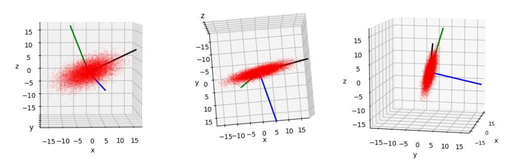
All axes are scaled and ticked in the same way. I have displayed colored lines indicating the directions of the eigenvectors, i.e. of the main axes of the ellipsoid. (The lines do not represent the lengths of the half-axes.) The blue main axis shows downwards in z-direction. The ellipsoid is longest along its black main axis and thinnest in the direction of its blue main axis.

Off topic: 3D axis-frames of Matplotlib very often do not represent the overlap and occlusion of objects in the 3D space correctly. For those who wonder how I got the z-order in the direction of the viewer right, please read about the option “computed_zorder=False” when creating a 3D subplot as in fig.add_subplot(131, projection=’3d’, computed_zorder=False). The right z-order can afterwards be set for the vectors [done with quiver()] and the scattered points [done with scatter()].

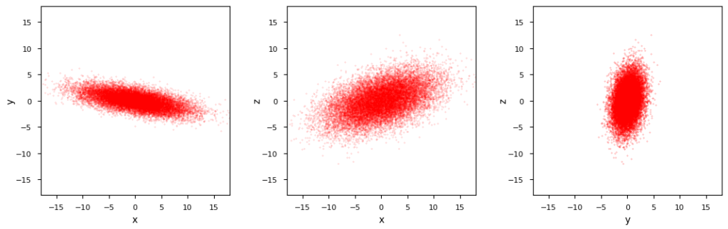
The resulting marginal BVDs are shown in the following plot:

Standard numerical methods like Numpy’s cov() reproduce the covariance matrix with an error of less than 4%. This gives us reliiable confidence ellipses:

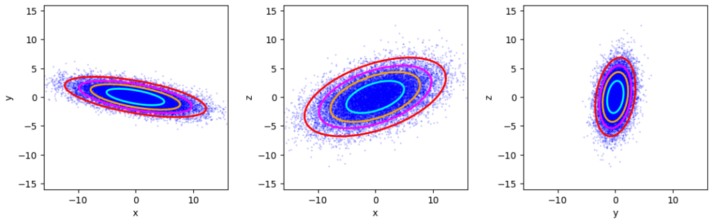
We see the already familiar fact that confidence ellipsoids and respective projected ellipses are concentrically arranged objects.

Two types of controlled perturbations

Creating controllable and directed disturbances of a regular MVD is an art of its own. I briefly discuss two steps to create (major) deviations from an ideal MVN:

1. Perturbation A: Applying systematic large and optionally asymmetric disturbances to points of outer layers beyond a defined Mahalanobis distance d_m,outer (normally chosen to fulfill d_m,outer > d_m,c). These disturbances are set to grow proportional to the original distance of the affected data points to the MVN’s center.
2. Perturbation B: Adding random and optionally both asymmetric and radius-dependent jitter noise to the coordinates of points in an inner core region of the original MVN (d_m ≤ d_m,c) .

Point (1) leads to the creation of a correlated bunch of “outliers” beyond d_m,outer.

Important note: It is easy to see that the order of the application of these (asymmetric) perturbations – A ahead of B or B ahead of A – will play a decisive role. If we first shift layers of the inner core and afterward apply an outer huge perturbation this may also affect points of the original inner core – which may then shrink significantly. In particular, if the perturbation regions overlap by choosing d_m,c ≥ d_m,outer.

Perturbation method A: Applying a direction dependent coordinate shift to outer points

This kind of perturbation is turned on only for points beyond a certain Mahalanobis distance of the original MND: d_m > d_m,outer.

We use a “disturbance direction vector” [DDV] attached to the center of the original MVN-distribution to indicate the direction of the perturbation. We then shift data points further away from the origin. We shift the points in proportion to their original distance from the center – in the direction of the DDV. To center the coordinate shift around the DDV-vector we can use a cosine function (or its square) to weigh the degree of disturbance by the angle between the position vector to a data point and the DDV.

This approach pushes points in the distribution’s outer regions systematically to greater distances – in the direction of the DDV. I.e. we create outliers in outer regions of the distribution – tearing both the center of the resulting distribution and its general shape into the DDV direction. The smaller we chose the border Mahalanobis distance d_m,outer, the stronger the directed dissolution effect will be. In addition, the correlations of the data points’ coordinates change significantly. This may lead to overall confidence ellipses which do not at all represent the orientation of the inner core of the distribution correctly.

Perturbation method B: Jitter – adding simple inner disturbances to coordinate values

We can manipulate the position of a data point by adding or subtracting statistical delta-values to its coordinates. To guarantee a remaining dense inner core of the overall distribution, the size of the perturbation will for our purposes be regulated by some simple factors and rules:

1. We generate a statistical jitter-factor f_jit with values in [-1., 1.] for each of the data points and each of their three coordinates.
2. We scale the perturbation of each coordinate by a fraction f_ract of a point’s distance d from the origin – but only for points up to a certain Mahalanobis distance d_m,c (describing an inner core; e.g. d_m,c = 1.7); this creates a perturbation p = f_jit * f_ract * d, growing in absolute value with the points’ distances from the origin. If we do not make f_ract too large, we keep up a centrally condensed distribution.
3. We apply an absolute maximum value p_max (|p| < p_max) for any perturbation. The maximum can e.g. be taken as some fraction of the smallest half-axis at a defined Mahalanobis distance d_m,limit < d_m,c (e.g. for d_m,limit = 1.5 ). This limits the coordinate perturbations for outer points.
4. We impose an optional asymmetry by selecting only one or two of the three coordinates for the disturbances and by using only positive (or only negative) jitter-factors. Alternatively, the disturbance direction can be defined by a directed vector. The change per coordinate direction would then be given by respective projections.

The 2nd point (b) is required to keep up a dense core. However, due to the distance dependency, it re-scales the extensions and proportions of the inner distribution. The 3rd limitation is required to avoid big absolute disturbances for points at large distances. The 4th point (d) also allows for a limited shift of the somewhat deformed inner core into a certain direction.

Together these rules give us a simple distance dependent and limited statistical jitter perturbation.

The value of robust covariance estimators

Let us assume that we have a distribution of data points with a centered inner core resembling a MVN. Let us further assume that the outer layers of the distribution stretch asymmetrically out to large distances and are not compatible with the MVN. As already mentioned, the outer points can be regarded as so called outliers from the perspective of the inner MVN-like core. Such outliers may have a big and drastic impact both on the center of the distribution and the orientation of confidence ellipsoids/ellipses. At least, when we determine the covariance matrix and the center of the full distribution with standard methods. Therefore, the covariance matrix of the overall distribution may not give us a proper idea of a similar matrix for the inner core and the properties of its confidence ellipses.

In such a situation, just calculating a covariance matrix via Numpy’s cov() or SciKit-Learn’s EmpiricalCovariance() functions for the whole distribution may give us orientations of confidence ellipses into the direction of the systematic perturbation. This direction would deviate from the orientation of respective ellipsoids/ellipses describing the inner core’s density distribution.

Now, you may say: Only take data points up to a certain Mahalanobis distance from the assumed correct center to calculate the covariance matrix. Well, this idea is accompanied by at least three problems for a given distribution:

1. How to guess a reasonable center of the inner core? In hundreds of dimensions?
2. The calculation of a (reasonable) Mahalanobis distance for data points in the inner part already requires a reasonably well estimated covariance matrix for the inner core of the distribution.
3. A covariance calculation which only regards inner points of an assumed MVN (residing within a d_m,c ) drastically underestimates the real values of the covariance matrix-elements of a respective full MVN having the same inner points. This has to be corrected by a factor (or factors ?) f_corr for the matrix elements depending on d_m,c.

To work around the first two problems, we can use so called “robust covariance estimators“. One example is an estimator build upon minimizing the determinant of the covariance matrix of a distribution by leaving out assumed outliers. Respective solvers have been build – the most prominent example is SciKit Learn’s function MinCovDet (). It works quire well, if the number of outliers does not dominate the distribution, i.e.: The distribution should still have a dense core approximating that of a MVN up to some distances around this center. MinCovDet creates a Python-object, which in turn provides us with a robust estimation of the distribution’s center and a respective covariance matrix.

For complicated cases and regarding a reasonable center, we can also guess a center of the distribution’s inner core ourselves (e.g. from plots), center the distribution accordingly and set a parameter “assume_centered=True” in the interface of MinCovDet.

Solution to the problem of a border of the inner MVN-core and a related cut off of respective numerical integrations

One can show that for one and the same cut off distance d_m,cutoff, the required correction factors f_corr are the same for different MVNs (in n dimensions) and for all elements of the covariance matrices. The factor is also dependent on the number of dimensions n:
f_corr = f_corr(d_m,cutoff, n).

You can create good values of correction factors f_corr(d_m,inner) numerically by comparing respective results of numerical integrations of the covariance integral of a full MVN and integrations over points of an inner part up to a given Mahalanobis distance, only. As said: One can prove that these correction factors are independent of the exact form of the MVN.

The mathematical proof is beyond the scope of this post; but experienced readers will not be surprised to hear that the factors depend on functions describing chi-square distributions with n degrees of freedom.

Hint: When you numerically create a list of correction factors for different values d_m,inner, you should cover a relative broad interval of small d_m–values (down to d_m = 1.0), just to be prepared for very limited compact inner cores containing only down to 50% of the data points.

Iterations to calculate the covariance matrix of an inner core

Let us now turn to an iterative method to calculate the covariance matrix describing the MVN which data points of an inner core approximate up to a cut off Mahalanobis distance d_m,c. If outer asymmetric layers are extended and contain many data points the robustly estimated covariance matrix may still describe the properties of the inner core wrongly. As most robust estimator methods systematically eliminate assumed outlier points and do so mainly for suspect outer points, these methods typically underestimate the size of the elements of the covariance matrix. In other more complicated cases we may get an overestimation.

After some extensive tests, I have found that these disadvantages can be compensated in parts by a nice trick that uses 3 basic steps plus additional iteration steps to find an improved estimate of the covariance matrix:

• Step 1: We first determine a robustly estimated cov-matrix cov_est (and a robustly estimated center mean_est, too) by using MinCovDet.
• Step 2: We determine a new corrected covariance matrix cov_corr and new center mean_corr by including only inner points up to a certain Mahalanobis distance d_m,inner. In this step an estimated Mahalanobis distance for inner points is calculated with the help of the previously estimated cov-matrix cov_est. We use the thereby selected inner points to determine the new mean_corr and cov_corr.
• Step 3: We correct the underestimated elements of cov_corr by applying our numerically determined correction factors fact_corr(d_m,inner); see above.
• Step(s) 4 (, m), optional: We iterate steps 2 and 3 multiple times, but this time by supplying the output cov_corr and mean_corr of the last iteration. I.e. we now set cov_est = cov_corr and mean_est = mean_corr as input data for calculating Mahalanobis distances and selecting inner points around mean_est. We, of course, use the same d_m,inner as before.

The final cov_corr and mean_corr are then used to construct confidence ellipses.

Note that the iteration both tries to correct the center and the orientation of the confidence ellipsoids by successively and systematically selecting new sets of inner points given by the changing cov_corr and respectively changing d_m-values.

How can we know that the iteration will move our estimated center mean_corr towards the inner core? Good question! In my experience the iteration will work as long as there is an overall density gradient in the outer layers, whose inverse would point inwards, i.e. grossly in the direction of the inner core. This is most often the case for datasets describing natural objects. In complicated cases you may have to help the robust estimator and the iterative process a bit by providing an artificial initial center and a large enough starting value for d_m,inner to sense a density gradient in the covered region.

The attentive reader has probably noticed another remaining problem: How to set d_m,inner when we do not know a reliable Mahalanobis distance for the size d_m,c of the core?

Well, while the optimal choice of d_m,inner depends on the size of the inner MVN-core in your data set, your ellipses will not turn out to become too wrong if you start with too small values of d_m,inner. The reason is that your correction factor f_corr will work anyway! As soon as we approach the inner core, the problem is more that for a too big estimate of d_m,inner ( > d_m,c ), you would include too many outliers in your computations. So, after a first convergence, also try out a rather small value and increase d_m,inner step-wise afterwards. Check after each step whether the axis inclinations, the size of the ellipses and their center positions start to change substantially with each step. Also use plots to verify our eventual choice. But keep in mind that sometimes the choice of an initial d_m,inner will also depend on the structure and density gradient variation in the outer layers. So be careful, not to destroy the basic convergence of the iteration by a too small initial value of d_m,inner.

The described iteration opens up a chance to find a better guess of the covariance matrix in cases for which even the robust estimation of the cov-matrix reacts to distant outliers. The convergence of the iteration and the eventual results should in any case be checked and verified – numerically, but also with the help of plots.

A first example to illustrate the capability of the suggested method

I will discuss test cases in detail in forthcoming posts. Just to give you a first impression what the iterative approach can do for you, I plot the characteristics of a rather extreme asymmetric perturbation of the initially defined MVN example:

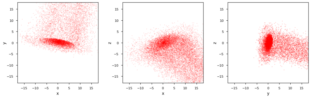
We see a strong asymmetric shift of outer layers in the direction of the smallest half axis of the original MVN. This leads to a long tail of points. Within the tail there is still an overall density gradient pointing outwards. An inner core with ellipsoidal shape still exists – in a somewhat shrunk and partially dissolved form, with its center a bit shifted into x,y-direction.

Of course a standard method to determine the covariance matrix of the whole deformed distribution reacts to the tail – both regarding a new center of the distribution and an elongated axis of the confidence ellipses in the tail’s direction:

Confidence ellipses according to Numpy’s cov()-function – for the whole distribution

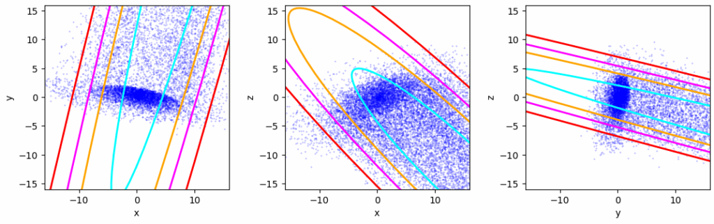
What about a robust estimator? Well, in the depicted case the disturbance is so extreme that it reacts, too, though less pronounced.

Confidence ellipses according to Scikit-Learns robust covariance estimator MinCovDet

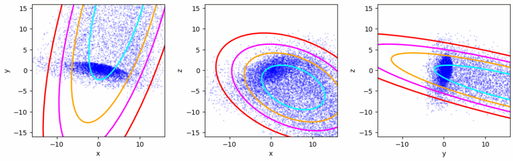
Obviously, both methods can not deliver a covariance matrix which would describe the properties of the remaining inner core. Note that this core still shows an overall ellipsoidal distribution with density increasing towards its center.

What does the iterative method give us after 7 iterations?

Confidence ellipses for the inner core derived by the suggested iterative method

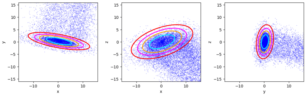
While the first 4 iterations did not deliver satisfying results, 2 additional iterations marked convergence and a last (7th) iteration corrected the orientations of the ellipsoid’s three axis a bit. More details will be shown and discussed in forthcoming posts.

Conclusion

It is a difficult task to compute confidence ellipsoids and respective ellipses of a dense, but limited, ellipsoidal and MVN-like core of a multidimensional data distribution with strongly asymmetric and extended outer layers. Even a robust estimator may not save us when the outer layers contain a significant number of points. In this post, I have suggested an iterative method to compute a reasonable covariance matrix for the inner core. This method can be automated. In forthcoming posts, I will discuss and show examples – also for a bigger number of dimensions.

Links and Literature

[1] R. Mönchmeyer, 2025, “Bivariate Normal Distributions – parameterization of contour ellipses in terms of the Mahalanobis distance and an angle”,
https://machine-learning.anracom.com/2025/07/07/bivariate-normal-distributions-parameterization-of-contour-ellipses-in-terms-of-the-mahalanobis-distance-and-an-angle/

[2] R. Mönchmeyer, 2025, “How to compute confidence ellipses – I – simple method based on the Pearson correlation coefficient”,
https://machine-learning.anracom.com/2025/08/02/how-to-compute-confidence-ellipses-i-simple-method-based-on-the-pearson-correlation-coefficient/

[3] R. Mönchmeyer, 2025, “How to compute confidence ellipses – III – 4 alternative construction methods”,
https://machine-learning.anracom.com/2025/10/21/how-to-compute-confidence-ellipses-iii-4-alternative-construction-methods/

[4] M. Hubert, M. Debruyne, 2009, “Minimum covariance determinant”, John Wiley & Sons,
https://wis.kuleuven.be/stat/robust/papers/2010/wire-mcd.pdf

[5] M. Hubert, M. Debruyne, P. J. Rousseeuw, 2017, “Minimum Covariance Determinant and Extensions”, arXiv:1709.07045v1,
https://arxiv.org/pdf/1709.07045

[6] [1] Carsten Schelp, “An Alternative Way to Plot the Covariance Ellipse”,
https://carstenschelp.github.io/2018/09/14/Plot_Confidence_Ellipse_001.html

[7] R. Mönchmeyer, 2025, “Properties of BVD confidence ellipses – I – constant limits and tangents in x- and y-direction during variation of the Pearson correlation coefficient”,
https://machine-learning.anracom.com/2025/08/07/properties-of-bvd-confidence-ellipses-i-constant-limits-and-tangents-in-x-and-y-direction-during-variation-of-the-pearson-correlation-coefficient/

[8] R. Mönchmeyer, 2025, “Properties of BVD confidence ellipses – II – dependency of half-axes on the correlation coefficient”,
https://machine-learning.anracom.com/2025/08/11/properties-of-bvd-confidence-ellipses-ii-dependency-of-half-axes-on-the-correlation-coefficient/