Ellipses via matrix elements – II – numerical tests of formulas

During the last posts, I have discussed properties of ellipses and ways to (re-) construct them from elements of a symmetric, invertible and positive-definite (2×2)-matrix, which defines a quadratic form. In the context of Machine Learning we often have to determine confidence ellipses from elements of a numerically determined variance-covariance matrix of statistical bivariate vector-distributions. Formulas relating the geometric properties of ellipses with matrix elements are very helpful to solve such problems. But the intimate relation between ellipses and certain types of matrices reaches beyond Machine Learning and statistics.

In this post I want to test some formulas presented in previous posts in this blog, namely

Post I: Ellipses via matrix elements – I – basic derivations and formulas,
Post II: Cholesky decomposition of an ellipse-defining symmetric matrix,

via respective numerical experiments performed with a Python program. We will in particular see that by observing certain rules for the determination of an ellipse’s rotation angle, we get a full agreement of re-construction methods based on an eigendecomposition of a matrix with methods based on Cholesky decomposition.

Suppositions, program elements, settings and tasks

We start with a symmetric, invertible (2×2)-matrix A_q that defines a quadratic form for an ellipse:

\[ \mbox{Ellipse, }\,\, {\mathbb{R}}^2 \,: \quad \pmb{v}_E^{\operatorname{T}} \circ \operatorname{\pmb{A}}_q \circ \, \pmb{v}_E \:=\: 1\,, \quad v_E \:=\: \begin{pmatrix} x_E \\ y_E \end{pmatrix} \tag{1} \]

\[ \operatorname{\pmb{A}}_q \:=\: \begin{pmatrix} \alpha & \beta/2 \\ \beta/2 & \gamma\end{pmatrix} \,, \tag{2} \]

\[ \begin{align} {\text{det}} \left( \operatorname{\pmb{A}}_q \right) \:=\: \alpha*\gamma \,-\, {1 \over 4}\, \beta^2 \:\gt\: 0 \,. \tag{3} \end{align} \]

Note that we have shown in post I that for a positive-definite matrix A_q which guarantees positive eigenvalues – and thereby positive lengths of the ellipse’s half axis – the matrix elements must furthermore fulfill

\[ \alpha \,\gt\, 0 \quad \land \quad \gamma \,\gt \, 0 \quad \land \quad \beta^2 \lt 4 \, \alpha \, \gamma \,. \tag{4} \]

Such a matrix A_q has eigenvalues λ_I and λ_II which determine the lengths of the ellipse’s half-axes h_I and h_II:

\[ \begin{align} \lambda_I \:&=\: {1 \over 2} \left(\, \left(\alpha \,+\, \gamma \right) \,-\, \left[ \beta^2 \,+\, \left(\gamma \,-\, \alpha \right)^2 \,\right]^{1/2} \, \right) \,, \tag{5} \\[10pt] \lambda_{II} \:&=\: {1 \over 2} \left(\, \left(\alpha \,+\, \gamma \right) \,+\, \left[ \beta^2 \,+\, \left(\gamma \,-\, \alpha \right)^2 \,\right]^{1/2} \, \right) \,. \tag{6} \end{align} \]

\[ h_I \:=\: 1 / \sqrt{\lambda_I}\,, \quad h_{II} \:=\: 1 / \sqrt{\lambda_{II}} \,. \tag{7}\]

Basic reconstruction of the ellipse by stretching and rotating a unit circle

The ellipse defined by A_q can be constructed by applying another (2×2)-matrix A_E on vectors defining a unit circle. A_E consists of (i) a stretching of vectors in x– and y-direction, which defines the longer and the shorter half-axis, and (ii) of a sub-sequent rotation by an angle Φ. The elements of A_E depend in a well defined way on the elements of A_q. The half-axes define the required scaling of vectors and Φ the rotation. Φ depends on α, β and γ and certain relations of these elements.

\[ \pmb{\operatorname{A}}_E \:=\: \pmb{\operatorname{R}}_{\phi} \circ \pmb{\operatorname{D}}_E \:=\: \begin{pmatrix} \lambda_1 & 0 \\ 0 & \lambda_2 \end{pmatrix} \circ \begin{pmatrix} \cos \phi & – \, \sin \phi \\ \sin \phi & \cos \phi \end{pmatrix} \,\,. \tag{8} \]

We “just” need to assign either λ_I to λ₁ and λ_II to λ₂ – or vice versa – and follow some rules to calculate Φ.

8 different cases, 4 core cases

In post I we have seen that we must potentially distinguish 8 different cases when we construct an ellipse from a given symmetric matrix A_q. The distinction was based on values of the matrix elements on one side and on the other side on an assumption regarding the question, which of the two perpendicular half-axis of the ellipse was the longer one, before we applied a rotation against the chosen Cartesian coordinate system. The reason is that the rotation angle Φ depends upon the latter assumption. The rules for determining the rotation angle were summarized in post I in form of a table:

Table 1 – determination of rotation angle Φ for different cases and helper angle ψ

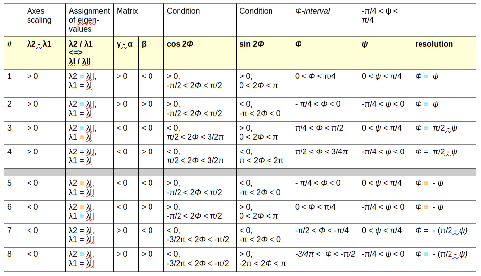
Table for determination of rotation angle of a matrix-defined ellipse

λ₁ and λ₂ mean eigenvalues controlling the lengths of the ellipse’s half-axes. See post I for more information. The helper angle ψ was given by

\[ \psi \::=\:\, {1 \over 2} \operatorname{arcsin} \left( {-\, \beta \over \left[ \beta^2 \, +\, \left( \gamma \,-\, \alpha \right)^2 \, \right]^{1/2} } \right) \,. \tag{9} \]

We saw, however, that 4 of the cases in the lower half of the table were equivalent to 4 other ones in the upper half. We claimed that the correspondence of cases is given by the following list of case equivalence :

List of corresponding, equivalent cases for identical elements of A_q

case #=7 <=> case #=1 ,
case #=8 <=> case #=2 ,
case #=5 <=> case #=3 ,
case #=6 <=> case #=4 .

We want to show with our numerical experiments that this indeed is the case.

Reconstruction methods and other elements of the Python program

Reference method 1: To test the prescriptions given by table 1 above, we need a kind of reference method for the re-construction of our ellipses. We found such a method in post II. There we saw that the very same ellipse given by could be created by applying a simple and distinctly defined linear transformation K_ch to vectors of a unit circle. K_ch is given as a lower triangular matrix coming from a Cholesky decomposition of the inverse [A_q]^-1 of A_q:

\[ \left[ \operatorname{\pmb{A}}_q \right]^{-1} \:=\: \operatorname{\pmb{K}}_{ch}\,\bullet\,\operatorname{\pmb{K}}_{ch}^{\operatorname{T}}\, . \tag{10} \]

In post II I have given formulas for computing the elements of K_c from the elements of A_q. We parameterize vectors v_c to the unit circle by 300 equidistant values of an angle θ in the following interval:

\[ \pmb{v}_{c} \,=\, \begin{pmatrix} \cos \theta \\ \sin\theta \end{pmatrix} \,, \quad 0\,\le\, \theta \,\le\, 2 \pi \,. \tag{11} \]

Reference ellipses are created by applying matrix K_ch to these vectors.

Method 2: Another part of the programs constructs ellipses by the help of a matrix A_E. The two options for the assignment of the eigenvalues λ_I and λ_II of A_q to the elements λ₁ and λ₂ of the stretching matrix D_E distinguishes the cases in the upper part of the table from he cases of the lower part – for otherwise identical values of α, β, γ.

Python code: The formulas given above and the rules in table 1 can easily be implemented with the help of a Python 3 program. Values of α, β and γ are statistically created within certain allowed ranges. I omit the code here, because it is trivial. Plots were all done with the help of Matplotlib.

Numerical tests

We perform the following tests:

Test 1: In a first test, I created multiple matrices A_q, whose elements got statistical values (within given intervals), but fulfilled our conditions (4). Furthermore, the created matrices covered all cases of table 1. In a first step I created respective ellipses by the reference method, i.e. with the help of K_ch. In a second step, I afterward calculated the eigenvalues of the different A_q matrices and assigned either h_I or h_II to the half-axes in x-direction and used the values as stretching factors of a diagonal matrix. Afterward, I determined the rotation angle Φ according to the rules of table 1, and set up the full matrix A_E. I eventually created the ellipses by applying A_E to vectors of a unit circle – and compared the results to those of the reference method.

Test 2: I again created cases which covered all of the conditions in the above table with the exception of the assignment of the eigenvalues to x- and y- half-axes. But this time I used the same values of α, β, γ for the corresponding cases. The expectation was that the two ellipses of corresponding cases would cover each other perfectly. This would indicate that we can always make the assignments

\[ \lambda_1 \,=\, \lambda_I \,, \quad \lambda_2 \,=\, \lambda_{II} \,, \tag{12} \]

and follow the rules in the upper part of the table – without loosing information or missing some special cases.

Plots for test 1

The following plots were created created for matrices with statistically chosen values

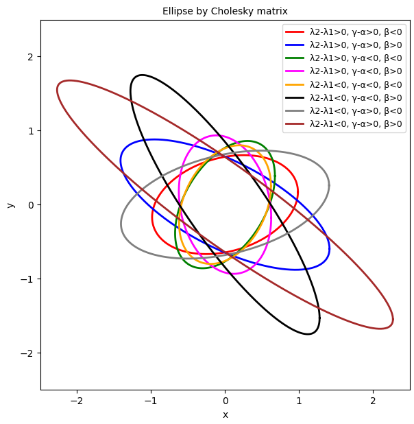
\[ \begin{align} &\text{Cases 1 to 4}: \quad \gamma \in [2., \, 3.], \quad \delta \in [1,0, \,1.9], \quad \alpha \,=\, \gamma \,-\, \delta , \quad \beta^2 \in [0, 4\,\alpha \, \gamma ] \,, \\[10pt] & \text{Cases 5 to 8}: \quad \alpha \in [2., \, 3.], \quad \delta \in [1,0, \,1.9], \quad \gamma \,=\, \alpha \,-\, \delta , \quad \beta^2 \in [0, 4\,\alpha \, \gamma ] \,. \end{align} \]

Plot 1.1 shows the result for ellipses created by the reference method, i.e. with matrix K_ch calculated from a Cholesky decomposition of [A_q]^-1.

Plot 1.1: Ellipses based on statistical data for the elements of A_q and Cholesky decomposition of [A_q]^-1

Plot 1.1 : Creation of ellipses with the help of a matrix from a Cholesky decomposition. — Plot 1.1 : Creation of ellipses with the help of a matrix from a Cholesky decomposition of the inverse of A_q.

Plot 1.2 shows the ellipses created with the help of a matrix A_E calculated from the elements of A_q. We first calculated the eigenvalues of A_q, determined angles ψ and Φ according to the rules in table 1, and derived matrix A_E from the gathered information.

Plot 1.2: Ellipses based on statistical data for the elements of A_q and a matrix A_E derived via the eigenvalues/eigenvectors of A_q

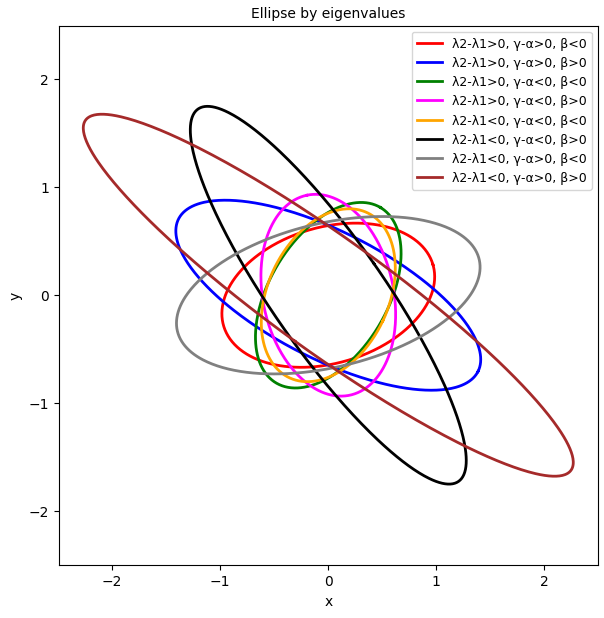
Plot 1.2 : Creation of ellipses with the help of the eigenvalues of the matrix Aq for a quadratic form — Plot 1.2 : Creation of ellipses with the help of the eigenvalues of the matrix A_q for a quadratic form

Up to invisible deviations due to numerical rounding the plots are identical. This shows that we can indeed use the eigenvalues of a matrix A_q and an angle determined by the rules of table 1 to reconstruct ellipses via a matrix A_E .

Plots for test 2

We now keep the matrix elements for the listed corresponding cases the same – and plot all 8 cases. This should, of course, give us only 4 plots from the reference method (same invertible, pos.-def. matrix => same decomposition!) . More interesting is the plot for the application of matrices A_E based on the eigenvalues of the matrices A_q. When we plot the cases 5 to 8 of table 1 later than cases 1 to 5, the plots for the cases in the lower part of table 1 should cover the plots for the upper cases completely. Only 4 ellipses should remain visible. We see this in plots 2.1, 2.2 and 2.3.

Plot 2.1: Ellipses based on statistical data for the elements of A_q and Cholesky decomposition of [A_q]^-1 – all 8 cases

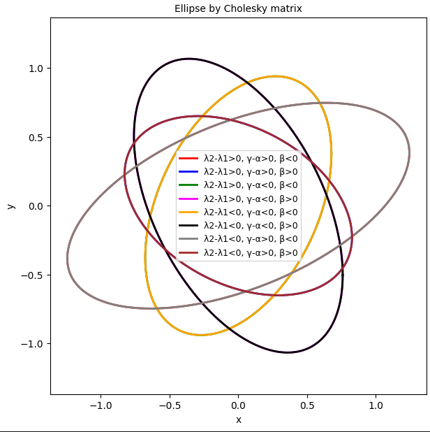
Plot 2.1 : Creation of ellipses with the help of a matrix from a Cholesky decomposition. Matrix elements were kept the same for corresponding cases in table 1.

This confirms our expectation that the ellipses from corresponding cases cover each other. Can we see how the covering of the ellipses happens? Plot 2.2 shows the cases 1 to 4, only.

Plot 2.2 Ellipses based on statistical data for the elements of A_q and Cholesky decomposition of [A_q]^-1 – the first 4 cases of table 1

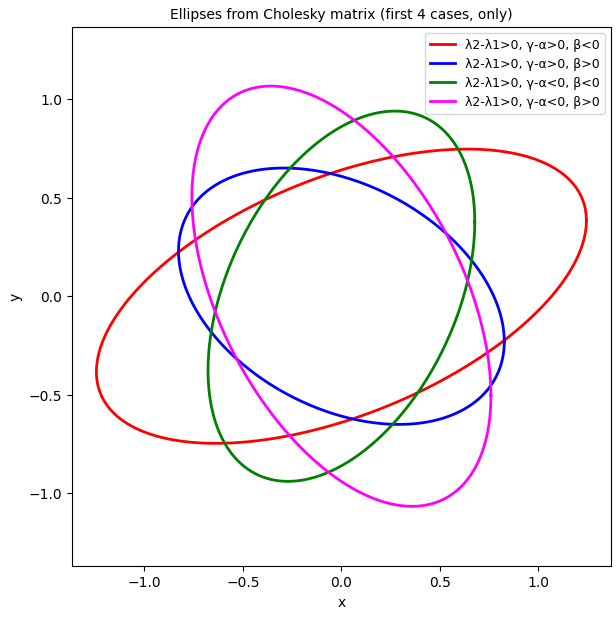
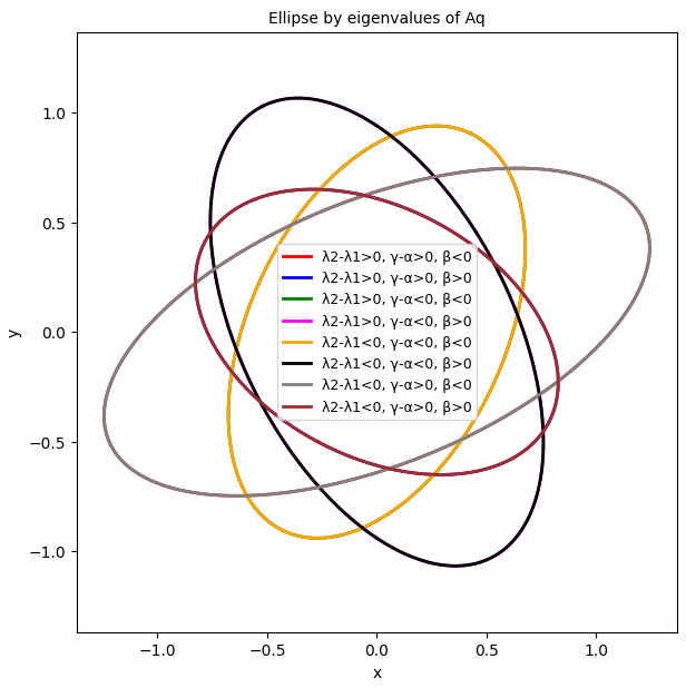
Plot 2.2 : Creation of ellipses with the help of a matrix from a Cholesky decomposition.(first 4 cases)

Now, comparing with plot 2.1, we see indeed that the ellipse for case 7 is identical with that of case 1. Case 8 is identical with case 2, case 6 with case 4 and case 5 with case 3. This result is confirmed in plot 2.3, which shows the results of the creation of the ellipses via a matrix A_E based on eigenvalues and angle Φ determined from A_q via the rules of table 1.

Plot 2.3 Ellipses based on statistical data for the elements of A_q and Cholesky decomposition of [A_q]^-1 – cases 5 to 8 of table 1 overlap corresponding cases 1 to 4

Plot 2.3 : Creation of ellipses with the help of the eigenvalues of the matrix Aq for a quadratic form. For identical matrix elements cases 4 to 8 have corresponding cases between 1 to 4. Corresponding ellipses overlap.

These findings confirm our claim in post I that for a given matrix we can always re-construct the ellipses by clinging to the cases in the upper part of table 1. I.e., we can simply assume

\[ \lambda_1 \,=\, \lambda_I \,, \quad \lambda_2 \,=\, \lambda_{II} \,, \]

and assign λ₁ the smaller eigenvalue – and thus align the larger half-axis of the yet un-rotated ellipse with the x-axis – without missing any “hidden” cases. The rotation angle Φ is automatically provided correctly if and when we follow the rules in the upper part of table 1.

Conclusion

In this post I have demonstrated via numerical experiments and respective plots that some of the claims and formulas stated in previous posts are correct. A given symmetric matrix A_q , which defines an ellipse via a proper quadratic form, provides two different methods to re-construct the respective ellipses:

Method 1: Use the lower triangular matrix K_ch of the Cholesky decomposition of [A_q]^-1 and apply K_ch to vectors defining a unit circle.
Method 2: Determine the eigenvalues of A_q and respective length-values of the ellipse’s half-axes. Align the longer half-axis with the x-axis and build a simple axis-parallel ellipse first. Afterward, apply a rotation to the ellipse, by an angle Φ calculated according to rules discriminating 4 basic cases for certain relations of the matrix elements.

Note that you should check some elementary conditions which the elements of a given matrix A_q must fulfill to guarantee an invertible, positive-definite matrix.

While our formulas in the mentioned posts are generally applicable, we will learn in a forthcoming post of this blog that there is yet another method to reconstruct contour ellipses of Bivariate Normal Distributions of vectors controlled by a symmetric covariance matrix.