In this post series we have a look at PyTorch dataloaders and Torchvision image datasets (downloaded via PyTorch modules). PyTorch DataLoaders retrieve batches of dataset elements and transfer them to neural networks [NN] on a computation device – e.g. a CUDA driven graphics card. A central dataset functions applies defined transformation operations to its elements. We analyze the impact of elementary transformations on the performance of training runs for small NN-models on a consumer GPU.
We saw that the parallelization of transform operations on the CPU via raising the “number of workers” of a PyTorch DataLoader object helped a lot. But, to challenge the GPU – a Nvidia 4060 TI – in the case of the MNIST dataset and a small CNN, we had to adjust the batch size to BS ≥ 128.
In this post we investigate whether it would help to perform basic transformation operations ahead of the network training and to preload the prepared data to the GPU. We will find a significant improvement. This in turn raises questions regarding augmentation operations on the CPU.
Previous posts:
- Post I: PyTorch / datasets / dataloader / data transfer to GPU – I – properties of some torchvision datasets
- Post II: PyTorch / datasets / dataloader / data transfer to GPU – II – dataloader too slow on CPU?
Results of previous posts and new objectives
Regarding PyTorch datasets we have seen that we can define a chain of transformation operations, which get applied whenever an indexed element of a PyTorch dataset is fetched. We have studied consequences of two elementary operations, ToTensor() and Normalize() – for the training of a small CNN with the MNIST dataset. In real world cases additional operations for normalization and image augmentation may have to be applied on the fly during the training of a NN-model. In a standard setup, such operations will be invoked on the CPU. Our question was whether this may lead to bottlenecks for the training of relatively small NN-models on a GPU.
We have found that for a given batch-size raising the number of dataloader workers [NW] helped. But for my given test system we came close to a limit with NW=6 workers. One reason was the growing load of my CPU (i7-6700K). However, we also saw a clear decline in the relative gain of performance when we increased NW for a given batch size BS.
We have also understood that we need to separate the impact of transformation operations form (1) the transfer of data batches to the GPU and (2) from other performance limiting factors.
Small NN-Models
One limiting factor can be the model itself, in combination with the GPU capabilities. (I assume that the NN-model has been transferred to the CUDA driven GPU-device.) I call a NN-model small, when the number of operations applied per batch does not cause a high continuous load on the GPU during the model training. The reason for a limited GPU load, of course, are the following:
- The batches must be processed sequentially for reasonable corrections of the NN-model parameters during training.
- There is a limit of useful parallelization for small batch sizes on the GPU.
Both factors lead to a limited GPU usage and GPU throughput. However, another factor in such a situation is the provision of batches. If all model related computations for a batch have been done, waiting for the next batch can press the performance under the theoretical limit. This may happen, if the batches do not arrive at the GPU with a sufficiently high frequency from the CPU. A too slow CPU (for a defined sequence of transformation operations) could become a bottleneck for small models on a modern GPU.
We would detect and overcome such a bottleneck with PyTorch by raising the number of workers NW and looking out for performance improvements.
(Note that the standard recipe with PyTorch is to continuously load data batches with a dataloader to the GPU, whilst with Keras/Tensorflow and simple default settings one may load all training data to the GPU ahead of the training run. )
Useless repetition of transformations
Another perfomance-limiting factor would be a meaningless repetition of elementary transformation operations. But, according to the analysis in the previous posts, this is exactly what happens in our case for our test operations ToTensor and Normalize. At least, if we followed PyTorch tutorials. These operations would be repeated for each image epoch for epoch. In addition, useless transformations from a tensor format to a PIL format and back to tensor format would occur.
Objectives
In this post we will try to find out what we can gain if and when we
- prepare required data tensors only once and ahead of the training to avoid unnecessary repetitions of basic operations during each of the training epochs,
- use a so called tensor-dataset,
- transfer the tensors them non-blockingly (i.e. asynchronously),
- preload all tensors to the GPU ahead of the training.
These steps will lead us to the maximum possible performance for a given model and batch-size. The result data of respective experiments will make it clear what we can maximally achieve by optimizing or circumventing the transformation processes in comparison to changing other conditions as e.g. the batch size.
Code snippets
In the preceding post I have provided code snippets which allow to perform controlled training runs for the purposes named above. I will just name the control parameters, which you have to change. The reader can derive the consequences by inspecting the simple code.
Using a tensor dataset
Our first major step will be to apply the transformations ToTensor() and Normalize() directly to the tensors coming as raw data of the Torchvision MNIST dataset. The most important of our control parameters to change is
b_TENSOR_DATASET = True .
When you look through the code in the preceding post, you will find that this basically leads to a sequence of the following operations
- pics = train_data.data.to(torch.float32).unsqueeze(1)
- pics2 = pics / 256.
- trans = transforms.Compose([ Normalize( (0.1302,), (0.3069,) ) ])
- pics3 = trans(pics2)
- tens_train_ds = torch.utils.data.TensorDataset(pics3, labels)
- train_tens_loader = DataLoader(tens_train_ds, batch_size=BATCH_SIZE_TRAIN, shuffle=b_SHUFFLE, num_workers=NUM_WORKERS, pin_memory=b_PIN_MEMORY, persistent_workers=b_PERSISTENT_WORKERS )
What we build here is a special dataset, which operates on PyTorch tensors, and a respective DataLoader object. If the dataset’s property “data” had not contained PyTorch tensors already, but data in other formats, we would have had to perform a transformation to tensors first. In the case of the MNIST dataset this is not required. We first set other parameters to the following values:
b_PIN_MEMORY = True, b_PERSISTENT_WORKERS = True.
We then vary the batch size, shuffling, the number of workers NW and in some cases a switch to asynchronous loading (see the next section). Afterward, we also preload fully prepared tensors to the GPU – more precisely to its VRAM. For result data see the tables and the images below.
Loading tensors asynchronously to the GPU
According to the code in the preceding post, we transfer batches to the NN-model (on the GPU) within the function training loop by using the batch tensor’s method “to(device)“. Normally, this operation is performed synchronously to the operations of the NN. I.e. the next batch is loaded when the preceding one has been processed by the model.
But, we have an option to transfer asynchronously – i.e. a tensor can be loaded while the previous one still is on its way through the NN-model. We achieve this by adding a parameter “non_blocking” and setting it to True [X: tensor for a batch of image data, y: tensor for a respective batch of label data]:
X, y = X.to(device, non_blocking=True), y.to(device, non_blocking=True)
Preloading the tensor arrays
In addition, in some runs, I preload the prepared tensor data to the GPU. This is controlled by the parameter
pics3.to(device) and label.to(device)
ahead of the training loop.
Note:
- The DataLoader object can nevertheless be built upon these preloaded tensors in the GPU’s VRAM.
- But: In this case the dataloader MUST be configured with standard parameters regarding the number of workers (num_workers = 0), pin_memory (= False), persistent_workers (= False). “num_workers = 0” means that the available main process for controlling the loading is used.
We will see that the pure transfer of prepared tensors to the (GPU-based) NN-model is a very efficient process.
Results
The following table summarizes results. The table is not filled completely. For experiments with preloaded tensors, we, of course, only can use the main loader process for the creation of batch tensors and thir transfer to the GPU. Such runs are marked by “NW = 0”.
I repeated some runs already done in the preceding post. Differences result from a different lower load due to background processes of other applications on my Linux system. The longest runs (i.e. the ones for small batch sizes) are in particular sensitive to background activities on the CPU. However and aside of singular run time values, the general tendencies seen in the last post were confirmed.
For runs with tensor datasets (“tens.-ds”) we distinguish between synchronous (“sync”) and asynchronous (“async”) data transfer.
| Batch Size |
NW | Shuffle | time sync, ds [sec] |
time async, ds [sec] |
time sync, tens.-ds [sec] |
time async, tens.-ds [sec] |
time preload, tens.-ds [sec] |
|---|---|---|---|---|---|---|---|
| 32 | 0 | yes | 458 | – | 150 | – | 145 |
| 32 | 0 | no | 450 | – | – | – | 144 |
| 32 | 1 | yes | 418 | 415 | 173 | 172 | – |
| 32 | 1 | no | 417 | 415 | 172 | 171 | – |
| 32 | 2 | yes | 252 | 252 | – | – | – |
| 32 | 3 | yes | 213 | – | – | – | – |
| 32 | 4 | yes | 212 | – | – | – | – |
| 32 | 6 | yes | 212 | 211 | 182 | 180 | – |
| 32 | 6 | no | 212 | – | 181 | 178 | – |
| 64 | 0 | yes | 389 | – | 83 | 82 | 81 |
| 64 | 0 | no | 380 | – | – | – | 81 |
| 64 | 1 | yes | 358 | 358 | 93 | 91 | – |
| 64 | 1 | no | 358 | – | 92 | 90 | – |
| 64 | 3 | yes | 158 | 158 | – | – | – |
| 64 | 4 | yes | 128 | 127 | – | – | – |
| 64 | 6 | yes | 120 | 119 | 96 | 95 | – |
| 64 | 6 | no | 120 | – | 95 | 94 | – |
| 128 | 0 | yes | 348 | – | 51 | 49 | 49 |
| 128 | 0 | no | 345 | – | – | – | 48 |
| 128 | 1 | yes | 332 | – | 53 | 50 | – |
| 128 | 1 | no | 329 | – | 53 | – | – |
| 128 | 4 | yes | 115 | – | – | – | – |
| 128 | 6 | yes | 85 | – | 55 | 51 | – |
| 128 | 6 | no | 85 | – | 54 | – | – |
| 256 | 0 | yes | 321 | – | 38 | 35 | 35 |
| 256 | 0 | no | 321 | – | – | – | 35 |
| 256 | 1 | yes | 312 | – | 40 | 36 | – |
| 256 | 1 | no | 312 | – | – | – | – |
| 256 | 4 | yes | 107 | – | – | – | – |
| 256 | 6 | yes | 80 | – | 40 | 36 | – |
The table is sorted with respect to the batch-size and the number of workers NW. The value 0 for the number of workers (NW = 0) represents cases for which default parameters of the DataLoader were used (as e.g. num_workers=0). This is of course the case for all runs with preloaded tensors.
The specific ordering in the table above obscures some trends a bit. Trends get clearer in the illustration below. Just click on it to get an enlarged version. For a compressed version leaving out certain minor important effects see below.
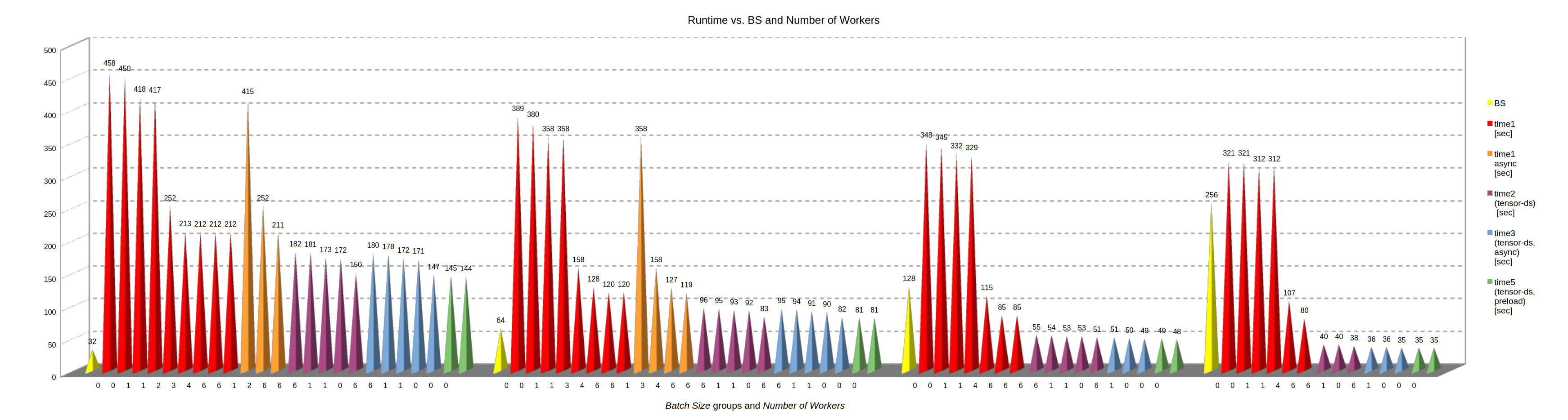
On the x-axis the number of workers NW is shown for each cone. If NW ≥ 1, memory pinning and persistent workers have been used.
What do the different cones mean?
- The grouping refers to certain batch sizes BS. The BS for each group is indicated by the respective leading yellow cone (32, 64, 128, 256).
- The red cones refer to standard runs with shuffling, synchronous transfer and standard unprepared datasets. I.e.: All transformations are done by an internal function (__get_item__) of the PyTorch dataset.
- The orange cones refer to similar runs as the red ones, but with asynchronous loading. The data just show that async loading has almost no impact for small batch sizes.
- The violet cones refer to runs with a tensor-dataset of fully prepared tensors. I.e., no transformations are performed on the CPU. Loading occurs synchronously.
- The blue cones refer to runs with a tensor-dataset of fully prepared tensors. I.e., no transformations are performed on the CPU. Loading occurs asynchronously. The differences in general are relatively small – i.e. below and around 10%.
- The green cones refer to runs with tensor-datasets built upon pre-loaded tensors. These runs use default parameters of the PyTorch DataLoader class (e.g. NW = num_workers = 0).
- All colors: Data for NW=0 refer to runs with default parameters for the DataLoader object. For double NW-number the first run is one with shuffling, the second one without shuffling.
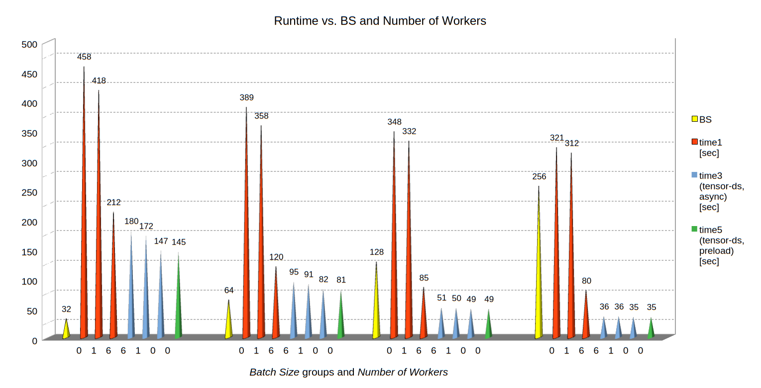
The illustration below is based on a condensed image with some data omitted:
Discussion
Impact of just one worker process (in addition to the main dataloader process) : We see that even NW = 1 (i.e. a parameter num_workers=1 for the dataloader) has an effect. The reason is that control tasks get separated from core tasks of the data processing ( batch creation and shuffling). The difference is significant for all batch sizes.
Impact of the number of workers for a standard dataset (performing transformation operations): The data above confirm that up to 3 or 4 workers we see significant improvements in the performance of runs with small batch sizes (BS < 64). But, we also find a clear tendency towards a plateau. This happens in the above case when batch handling and provision by the CPU runs into a limit. This limit may depend on the number of available CPU cores and overhead regarding general Linux process assignment to cores.
For large batch sizes, BS=128 or BS=256, however, raising the number to NW=6 helped significantly – and improved performance by more than 25%. Hence:
Rule 1: For standard Torchvision datasets, small batch sizes and small NN-models, it is worth trying to raise the number of workers – until you hit a performance limit of CPU.
Impact of using a tensor-dataset of prepared tensors: One of the striking results in the above data is that preparing the required tensors completely ahead of a training run and using a tensor-dataset results in a substantial acceleration – independent of the batch size BS.
Reason: The data preparation reduced the tasks of the DataLoader to the creation of batches and their transfer to the NN-model. These remaining tasks, obviously, are done by very efficient processes (index juggling, data to the GPU). Hence:
Rule 2: Prepare tensors for your image data as far as possible. Use tensor-datasets. And: Try to perform augmentation operations on the GPU.
Impact of the number of workers for a tensor-dataset of prepared tensors: In this case it seems that using more than just 1 worker only creates unnecessary overhead. Actually, we get an optimal performance for just using standard main dataloader process, i.e. for NW=0.
Rule 3: If you use a tensor-dataset of fully prepared tensors do not use multiple workers. Set NW=0 – and leave everything else to the main loader process.
Impact of asynchronous loading: Asynchronous loading is giving us improvements of at maximum 10%, only. The effect is significant for larger batch sizes, only.
Impact of shuffling: All in all a minor factor. We see some small run-time differences for small batch sizes and a small number of workers. But even for such runs the differences are below 1% and drastically shrinking with growing batch size. This can be explained by the fact that data shuffling is only index juggling.
Impact of preloading: Preloading data to the GPU may give us another 10% boost in comparison to runs with synchronous loading. However, for BS ≥ 128 the additional gain is small in comparison to runs with asynchronous loading.
Impact of the batch size: The batch size BS has a major impact on the overall performance. This is due to a much better usage of the GPU and its parallel units. This in turn requires a continuous supply of the larger batches on still relatively small timescales. So, for larger batch sizes and standard datasets of unprepared tensors, we expect more help from an increased number of workers on the GPU.
Note that for our test case we come close to the performance limit of the GPU with a batch size of BS=256. Therefore, the run with a tensor-dataset of prepared tensors marks a performance limit for our MNIST test case. It would be interesting to see what this limit looks like for the same test case, but using Keras with a Tensorflow 2 backend vs. a PyTorch backend.
CPU and GPU load
The following table summarizes some information on the CPU load and the GPU load for runs with shuffling and synchronous transfer. With asynchronous transfer, prepared tensors, NW=0 and BS ≥ 128 we get close to the data for preloaded tensors.
| Batch Size |
NW | Tensor dataset prepared |
Tensor dataset preloaded |
Avg. CPU load [%] |
Avg. GPU load [%] |
Avg. GPU power [Watt] |
|---|---|---|---|---|---|---|
| 32 | 1 | no | no | 24 | 13 | 35 |
| 32 | 6 | no | no | 53 | 27 | 48 |
| 32 | 1 | yes | no | 28 | 32 | 53 |
| 32 | 0 | yes | yes | 18 | 38 | 58 |
| 64 | 1 | no | no | 13 | 20 | 36 |
| 64 | 6 | no | no | 74 | 36 | 57 |
| 64 | 1 | yes | no | 30 | 45 | 70 |
| 64 | 0 | yes | yes | 17 | 49 | 77 |
| 128 | 1 | no | no | 12 | 19 | 39 |
| 128 | 6 | no | no | 90 | 44 | 72 |
| 128 | 1 | yes | no | 32 | 72 | 98 |
| 128 | 0 | yes | yes | 18 | 74 | 101 |
| 256 | 1 | no | no | 13 | 19 | 39 |
| 256 | 6 | no | no | 88 | 45 | 76 |
| 256 | 1 | yes | no | 29 | 91 | 126 |
| 256 | 0 | yes | yes | 18 | 99 | 138 |
We see that we can drive the GPU load up to almost 100% on my consumer card. Regarding total energy consumption one also has to take into account the runtime. Overall energy consumption gets smaller with shorter run-times: 138W x 35s = 4830Ws vs. e.g. 101W x 50s = 5050Ws vs. e.g. 58W x 145s = 8410Ws .
Conclusion
In this post, I tried to show that it is important to use dataloader and dataset parameters reasonably to utilize the potential performance of a given ML-system optimally with PyTorch. This is in particular true for small NN-models. The results of the experiments discussed above have shown the following:
For small NN-models it is worthwhile to balance CPU- and GPU-load for standard PyTorch datasets and unprepared image data. The number of workers for a PyTorch dataloader has to be chosen carefully and in relation to the batch size as well as to the CPU’s capabilities. One should in addition try to apply elementary transformation operations to the image data ahead of the training – as much as possible. For prepared tensors use a tensor-dataset. In case of tensor-datasets for fully prepared tensors use default parameters for your your PyTorch DataLoader object with num_workers=0. If possible, preload fully prepared tensors to the GPU.
The batch size for your training runs must be chosen carefully. Note that the batch size may have an impact on more than just performance for certain NN-models. It can influence convergence – especially if you turn to modelling learning rates and other hyper-parameters for super-convergence.
The results raise some questions about image augmentation, which I will discuss in the next and final post of this series.
Stay tuned …