For an old fan of Tensorflow2 it is somewhat satisfactory to notice that some problems also exist in analogous form in a PyTorch environment.
Anyone who has worked with visual data knows that one needs to modify, augment and transform the image data and then load them from some storage under CPU control to the GPU’s VRAM before or during the training of a neural network [NN]. On systems with only a few GB of VRAM we may be forced to provide images batch after batch to the GPU to keep the VRAM consumption on the GPU within acceptable limits. This is what data-pipelines do for us.
Some of TF2- related pipeline tools gave me a headache in the past, because under certain conditions they were painstakingly slow compared to what happened on the GPU. In particular for relatively small NN-models and small batches of data. This kind of potential mismatch between CPU and GPU capabilities also came up with PyTorch on my (relatively old) Linux systems. And some readers may have experienced similar problems on Google’s Colab service, too.
With this and the next 3 posts, I want to describe some recipes for loading data faster into the GPU. Recipes, which I found spread over Internet forums. In particular, I will have a look at the extreme case of loading all image data to the GPU ahead of any training operations. This sets a kind of limit for other measures. In this regard you can look at this post series also as a test of the graphics card (here a Nvidia RTX 4060 TI) and the PyTorch framework.
Addendum, 03/24/2025: After having tested the performance of Keras 3 with the PyTorch backend, the results of my present post series got even more interesting: The tests showed that one may achieve a better overall performance with a pure PyTorch approach than with Keras and a tensorflow backend. I will write about this topic soon.
I am just a beginner with PyTorch, so experienced users may just look with a pitying view at these three posts. But, I hope the contents may help other PyTorch beginners … To keep things simple I take the MNIST and FashionMNIST datasets as examples – although they have some special characteristics. One property is that they are grey images. This means that respective data may come without the usual 3 color layers.
In this first post we look a bit closer at some properties of typical torchvision datasets. This will help us later to understand what a dataloader object does and how we can transfer all image data of such a set directly to the GPU. I assume that the reader is familiar with the fact that data handling on a GPU requires that we provide the data in form of tensors, i.e. array-like objects of a special format suited for GPU operations.
The data property of Dataset objects for MNIST and FashionMNIST
Let us first look at the interface for downloading and using an available dataset for images. Below some code for FashionMNIST:
import torch
import torch.nn as nn
import torch.nn.functional as F
import torch.optim as optim
from torch.utils.data import DataLoader
from torchvision import datasets, transforms
from torchvision.transforms import ToTensor, Normalize, Compose
import matplotlib.pyplot as plt
from PIL import Image
# -------------------------------
# Path to Fashion MNIST data - this is were the dataset gets stored
root = '/mnt_ramdisk/FashionMNIST_data/'
# Load the data (if necessary)
train_data = datasets.FashionMNIST(root=root,
                               train=True,
                               download=True,
                               transform=Compose([
                                   ToTensor()
                               ])
)
print(train_data.__len__)
print()
print()
test_data = datasets.MNIST(root=root,
                           train=False,
                           download=True,
                           transform=Compose([
                               ToTensor(),
                           ])
)
print(test_data.__len__)
Note that datasets are provided by the package “torchvision“.
Obviously, one can define the path where to store the data. And we can define a chain of transformation operations, which shall be applied to the elements of the dataset. In the case above, we are not too astonished that the ToTensor -function appears as an element in this chain. We could also have supplemented normalization or augmentation operations. In this post, I leave such steps out for the sake of simplicity. But see the next posts in this series for an inclusion of a data normalization.
The definition of a dataset object looks promising. But how to break the data up into batches and how to transfer them to a NN-model? To answer these questions, most introductory documentations now directly turn to the application of a dataloader onto the dataset object. A dataloader object will handle further processing of the data for us. But, such a straightforward line of argumentation may leave the interested ML-developer with some open points. There are 3 points which I did not understand by following the usual path of available PyTorch documentation:
- Datasets may well have their own policies of in what format the raw data of the set are downloaded and saved in one of the target folders on your Linux system. Even the standard documentation of basic and specific classes for pytorchvision datasets (as e.g. the MNIST dataset) focuses on the class’s methods and not on its properties. A clear information about the property containing the raw data and their format is often lacking.
- The rules for certain obligatory functions of a standard Torch dataset class must, of course, be fulfilled by the classes for specific datasets. E.g., a method __getitem__() is always required. One understands that this function provides image and label data – but their format has to be guessed, too.
- Another point which remains somewhat obscure is the question when and how the transformations prescribed by some “transform”-settings in the dataset’s interface are applied.
All three points become, however, much clearer when one looks at the source code of a dataset class. And the information there opens up for a controlled option to load some datasets completely to the GPU.
For MNIST you find the source code here. First, note the central statement in the __init__ () function there.
self.data, self.targets = self._load_data()
So, in these cases we will find some data in the properties “data” and “target” of a concrete object instance of this class. Reading a bit in the code makes it clear that “data” are the training data, in case we choose a parameter value train=True. In case train=False we get label data. The respective property is called “targets“.
Ok, let us look at what kind of data format we actually get after having run the above statements:
print("ds shape = ", train_data.data.shape)
-------------------------------------------
ds shape =  torch.Size([60000, 28, 28])
print(train_data.data[1])
-------------------------------------

tensor([[  0,   0,   0,   0,   0,   1,   0,   0,   0,   0,  41, 188, 103,  54,
          48,  43,  87, 168, 133,  16,   0,   0,   0,   0,   0,   0,   0,   0],
        [  0,   0,   0,   1,   0,   0,   0,  49, 136, 219, 216, 228, 236, 255,
         255, 255, 255, 217, 215, 254, 231, 160,  45,   0,   0,   0,   0,   0],
...
[  0,   0,   0,   0,   0,   1,   0,   0, 139, 146, 130, 135, 135, 137,
         125, 124, 125, 121, 119, 114, 130,  76,   0,   0,   0,   0,   0,   0]],
       dtype=torch.uint8)
We take to notice that the data residing in train_data.data are already tensor objects.
So, if these data fulfilled dimension expectations of a NN-model, we could load them directly into the GPU. However, the raw data for MNIST/FashionMNIST do not fulfill such requirements. The reason is that they are gray scale images – and for a better download performance the tensors were squeezed by the responsible PyTorch team. Which is quite understandable. So, the downloaded tensors lack a dimension for the usual color layers. A dimension for indexing color layers is, however, a standard requirement that image tensors fed into the input layers of NNs must fulfill.
PIL image data vs dataset.data
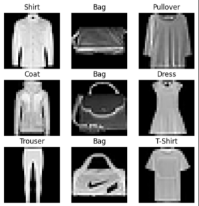
Now, you may answer that we actually do get conventional image data from a dataset as the following example code from a Pytorch tutorial shows:
labels_map = {
    0: "T-Shirt",  1: "Trouser",  2: "Pullover", 3: "Dress",
    4: "Coat",     5: "Sandal",   6: "Shirt",    7: "Sneaker",
    8: "Bag",      9: "Ankle Boot",
}
figure = plt.figure(figsize=(6, 6))
cols, rows = 3, 3
for i in range(1, cols * rows + 1):
    sample_idx = torch.randint(len(train_data), size=(1,)).item()
    img, label = train_data[sample_idx]
    figure.add_subplot(rows, cols, i)
    plt.title(labels_map[label])
    plt.axis("off")
    plt.imshow(img.squeeze(), cmap="gray")
plt.show()
The result looks like:
What happens under the hood of our dataset-object when we call an indexed element or item of the dataset?
img, label = train_data[sample_idx]
Another question, which also comes up, is: Why is the call of the squeeze()-method required when calling imshow() of Matplotlib ?
We find information about what happens during the retrieval of an indexed element in the code of the “__get_item__” – function of the dataset class, which actually provides the objects “img” and “label” in the above code :
def __getitem__(self, index: int) -> Tuple[Any, Any]:
        """
        Args:
            index (int): Index

        Returns:
            tuple: (image, target) where target is index of the target class.
        """
        img, target = self.data[index], int(self.targets[index])

        # doing this so that it is consistent with all other datasets
        # to return a PIL Image
        img = Image.fromarray(img.numpy(), mode="L")

        if self.transform is not None:
            img = self.transform(img)

        if self.target_transform is not None:
            target = self.target_transform(target)

        return img, target
Can we check this in more detail? Well, we just have to repeat the internal steps of __get_item__ and apply them e.g. to elements of train_data.data :
img = train_data.data[1]
img2 = Image.fromarray(img.numpy(), mode="L")
print("Info for img2 :")
print(img2)
print()
trans = transforms.Compose([ ToTensor(), ])
img3 = trans(img2)
print("Info for img3 :")
print("Shape imgg3 : ", img3.shape)
print(img3)
The output of this code snippet is :
Info for img2 :
<PIL.Image.Image image mode=L size=28x28 at 0x2FE587A3F1D0>

Info for img3 :
Shape imgg3 :  torch.Size([1, 28, 28])
tensor([[[0.0000, 0.0000, 0.0000, 0.0000, 0.0000, 0.0039, 0.0000, 0.0000,
          0.0000, 0.0000, 0.1608, 0.7373, 0.4039, 0.2118, 0.1882, 0.1686,
          0.3412, 0.6588, 0.5216, 0.0627, 0.0000, 0.0000, 0.0000, 0.0000,
          0.0000, 0.0000, 0.0000, 0.0000],
...
 [0.0000, 0.0000, 0.0000, 0.0000, 0.0000, 0.0039, 0.0000, 0.0000,
          0.5451, 0.5725, 0.5098, 0.5294, 0.5294, 0.5373, 0.4902, 0.4863,
          0.4902, 0.4745, 0.4667, 0.4471, 0.5098, 0.2980, 0.0000, 0.0000,
          0.0000, 0.0000, 0.0000, 0.0000]]])
This shows us what the dataset object internally does, when we fetch an indexed tuple element from it:
- In a first step it picks e.g. the respective element of the original tensor data (uint8) and turns it into a Numpy array. The Numpy array in turn is transformed into a PIL image. PIL images work with floats in the range [0.0, 1.0] to define pixel values.
- In a second step the chain of transformation operations is applied to the image’s float data. In our simple case the PIL format is turned into an image data tensor of the form [C, W, H] (with C: color channels, W: Width, H: Height). For our gray-scale MNIST images we get a shape of [1, 28, 28].
The second step explains why we we must use the squeeze-method before calling imshow(). __get_item__ provides a PIL image, only, if we had not defined a transformation to a tensor. Of course, we could have used the PIL image data directly for plotting. But as our specific train_data set also got transformation operations defined (via its “transform”-parameter), __get_item()__ produces a full fledged tensor. Applying the squeeze operation leads to an understandable simple 28×28 array input for plt.imshow().
Note: If you had not requested a transformation to a tensor when you defined the dataset, you could have directly provided the PIL image data to plt.imshow().
The important point for further analysis is that a PyTorch dataloader-object iterates over the data of a PyTorch dataset. Whilst doing so, it uses the method “__get_item__” of the dataset-object to provide output data, which can be sent to the GPU. The application of a dataloader and its cooperation with a simple NN-model (on a GPU) is the topic of the next post.
Conclusion
In this post we have seen that at least some available Torchvision datasets deliver their data already in a basic PyTorch tensor format. We have to refer to the “data“-property of the instantiated dataset object to access the respective tensor array. However, the basic image tensors do not always fit the standard expectations for image tensors by NNs. This is e.g. the case for gray images like the ones used in the usual MNIST and FashionMNIST datasets.
Defining a transformation chain including ToTensor() for the dataset’s parameter “transform” solves this problem. Such transformations are applied to the tuples (img, label) which we get when we call an indexed element of the PyTorch dataset. If and when we request a ToTensor() -transformation for both, the output tuple will consist of tensors usable for NN-models. Otherwise we would get image data in the PIL format and a label in an appropriate non-tensor format.
A visualization of the tensor image data of a requested dataset element requires an application of the squeeze-function to get a format which can be handled by matplotlib.
In the next post of this series
PyTorch / datasets / dataloader / data transfer to GPU – II – dataloader too slow on CPU?
we will investigate how a PyTorch dataloader works with a PyTorch dataset. We will also discuss which parameters have a major impact on the dataloaders performance during the training of a NN-model on a GPU.
Stay tuned …
Links
Code for MNIST dataset: https://pytorch.org/ vision/0.21/ _modules/ torchvision/ datasets/ mnist.html#MNIST
Tutorial for datasets and dataloader: https://pytorch.org/ tutorials/ beginner/ basics/ data_tutorial.html
Addendum, 14.03.2025 – How to get the value of a label?
A reader has asked ho to get the value of a label from the downloaded tensors of a dataset. You find the labels of images, which you may need for the training of a discriminator NN, in the property “dataset.targets” – also in tensor form.
This tensor has in the case of MNIST / FashionMNIST a dimension of zero – it actually is a number.
To use the labels outside of the GPU you have to call the item() method of the tensor object. See the following example, which produces a plot of a certain image (with index 15):
labels_map = {
    0: "T-Shirt",  1: "Trouser",  2: "Pullover", 3: "Dress",
    4: "Coat",     5: "Sandal",   6: "Shirt",    7: "Sneaker",
    8: "Bag",      9: "Ankle Boot",
}
idx = 15
img = train_data.data[idx]
img2 = Image.fromarray(img.numpy(), mode="L")
label = train_data.targets[idx].item()
labels_map = {
    0: "T-Shirt",  1: "Trouser",  2: "Pullover", 3: "Dress",
    4: "Coat",     5: "Sandal",   6: "Shirt",    7: "Sneaker",
    8: "Bag",      9: "Ankle Boot",
}

# Plot the image
figure = plt.figure(figsize=(4, 4))
cols, rows = 1, 1
for i in range(1, cols * rows + 1):
    figure.add_subplot(rows, cols, i)
    plt.title(labels_map[label])
    plt.axis("off")
    plt.imshow(img2, cmap="gray")
plt.show()