Multivariate Normal Distributions – II – Linear transformation of a random vector with independent standardized normal components

In Machine Learning we typically deal with huge, but finite vector distributions defined in the ℝⁿ. At least in certain regions of the ℝⁿ these distributions may approximate an underlying continuous distribution. In the first post of this series

Multivariate Normal Distributions – I – Basics and a random vector of independent Gaussians

we worked with a special type of continuous vector distribution based on independent 1-dimensional standardized normal distributions for the vector components. In this post we apply a linear transformation to the vectors of such a distribution. We restrict our present view onto transformations which can be represented by invertible quadratic (n x n) matrices M with constant real valued elements.

We will find that the resulting probability density function for the transformed vectors y = M • z are controlled by a symmetric invertible matrix Σ. These probability functions all have the same functional form based on a central product y^T • Σ^-1 • y. This result encourages a common definition of the corresponding vector distributions. We will call the resulting distributions “non-degenerate multivariate normal distribution“. They form a sub-set of more general multivariate normal distributions ([MNDs] or [MVNs]).

In this post I will closely follow a line of thought which many authors have published before. A prominent example is Prof. Richard Lockhart at the SFU, CA. See the following links to his lecture notes:

Any errors and incomplete derivations are my fault. Below I will use the abbreviation “pdf” for “probability density function”. Forthcoming posts we will deal with more general (n x m)-matrices and also singular, non-invertible (n x n) matrices.

Probability densities of random vectors with independent components

In the last post we introduced random vectors to represent certain statistical vector distributions. A random vector maps an object population to a distribution of vectors in the ℝⁿ by a statistical process. So far we have regarded random vectors having independent normal random variables (maps to ℝ) as components. I.e. the distribution of the values of a chosen component of the (densely populated) vector distribution could be described by a continuous 1-dimensional Gaussian probability density function. We have distinguished a normalized random vector W from a standardized one, which we named Z, and used the following notation to indicate that the related distributions represented special cases of MVNs:

$\begin{align} W_j \,\sim\, \mathcal{N}_1 \left( \mu_j,\,\sigma_j^{2} \right), & \quad \pmb{W} \,\sim\, \pmb{\mathcal{N}}_n \left(\pmb{\mu}_w,\, \pmb{\Sigma}_{\small W} \right) \\ \quad Z_j \,\sim\, \mathcal{N}_1 \left( 0, \,1 \right), &\quad \pmb{Z} \, \sim \pmb{\mathcal{N}}_n \left( \pmb{0}, \, \pmb{\operatorname{I}} \right) \end{align}$

Remember that the probability density functions g_w(w) and g_z(z) for W– and Z-related distributions of vectors w and z

$\pmb{w} \,=\, \left( w_1, w_2, \cdots, w_j, \cdots, w_n \right)^T, \quad \pmb{z} \,=\, \left( z_1, z_2, \cdots, z_j, \cdots, z_n \right)^T$

could be written as

$\begin{align} g_{\small W}(\pmb{w}, \pmb{\mu}_w, \pmb{\operatorname{\Sigma}}_{\small W}) \, &= \, {1 \over \sqrt{(2\pi)^n} } \, {\large e}^{ – \, {\Large 1 \over \Large 2} \left( \Large \pmb{w} – \Large \pmb{\mu}_w \right)^{\Large T} \, \bullet \,\, \pmb{\operatorname{ \Large \Sigma }}_{\small W}^{\Large -1} \bullet \, \left( \Large \pmb{w} – \pmb{\mu}_w \right) } \\ g_{\small Z}(\pmb{z}, \pmb{0}, \pmb{\operatorname{I}} ) \, &= \, {1 \over \sqrt{(2\pi)^n} } \, {\large e}^{ – \, {\Large 1 \over \Large 2} \left( {\Large \pmb{z}^T} \, \bullet \, {\Large \pmb{z}} \right) } \end{align} \, .$

It is easy to see that the contour-hypersurfaces of the probability density of the Z-distribution is given by surfaces of n-dimensional spheres.

Application of a linear, invertible transformation onto a random vector

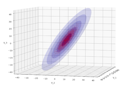
In this post we look at a random vector Y which results in target vectors y ∈ ℝⁿ that are related to target vectors z ∈ ℝⁿ of our standardized random vector Z by a linear transformation:

$\pmb{Y_N} \,=\, \left(Y_1, \, Y_2, \, ….., \, Y_n \right)^T \: = \: \pmb{\operatorname{M}}_{\small Y} \, {\small \bullet} \, \pmb{Z} + \pmb{\mu}_y$

The interpretation is that any vector z belonging to the Z-based distribution is transformed by M_y, i.e.: Any vector z of the distribution generated by Z would be transformed into y = M_y • z + μ_y. The following plot shows the result of such a transformation for a particular matrix:

We assume that the matrix M is invertible. I.e. for the (n x n) matrix M_y exists a matrix M_y^-1, such that

$\pmb{\operatorname{ M }}_{\small Y} \, {\small \bullet} \, \pmb{\operatorname{ M }}_{\small Y}^{-1} \,=\, \pmb{\operatorname{ I }}$

(Other cases will be handled in one of the forthcoming posts.) We then can write

$\pmb{y} = \pmb{\operatorname{M}}_{\small Y} \, {\small \bullet} \, \pmb{z} + \pmb{\mu_y} \,\, \Rightarrow \,\, \pmb{z}= \pmb{\operatorname{M}}_{\small Y}^{-1} {\small \bullet} \left( \pmb{y} – \pmb{\mu_y} \right)$

We note the following relations (in a somewhat relaxed notation, both with respect to the bullets marking matrix multiplications and the random vectors):

$\pmb{Z} \: = \: \pmb{\operatorname{M}}_{\small Y}^{-1}(\pmb{Y_N} \,-\, \pmb{\mu}_y)$

${\partial\pmb{Y_N} \over \partial\pmb{Z}} \, = \, \pmb{\operatorname{M}}_{\small Y}\, , \quad {\partial\pmb{Z} \over \partial\pmb{Y_N}} \, = \, \pmb{\operatorname{M}}_{\small Y}^{-1} \\ \operatorname{det}\left(\pmb{\operatorname{M}}_{\small Y}^{-1}\right) \,=\, \left(\operatorname{det}\left(\pmb{\operatorname{M}}_{\small Y}\right)\right)^{-1}.$

The last relation is basic Linear Algebra [LinAlg]. See e.g. here.

Transformation of the probability density

How does our probability density function g_z(z) transform? Remember that it is not sufficient to just rewrite the coordinate values in the density function. Instead we have to ensure that the product of the local density times an infinitesimal volume dV must remain constant during the coordinate transformation. Therefore we need the Jacobi-determinant of the variable transformation as an additional factor. (This is a basic theorem of multidimensional analysis for injective variable changes in multiple integrals and the transformation of infinitesimal volume elements).

For a linear transformation (like a rotation) the required determinant is just det(M_y) = |M_y|. Therefore:

$g_{\small Y}(\pmb{y})\,dV_y \:=\: g_{\small Z}(\pmb{z}(\pmb{x}))\,\left|\pmb{\operatorname{M}}_{\small Y}\right|dV_z \, \Rightarrow \, g_{\small Y}(\pmb{y}) \,=\, {1 \over \left|\pmb{\operatorname{M}}_{\small Y}\right|} \, g_{\small Z}(\pmb{z}(\pmb{y})) \, .$

Thus

$g_{\small Y}(\pmb{y}) \, = \, {1 \over \left|\pmb{\operatorname{M}}_{\small Y}\right|} \,*\, g_{\small Z}(\pmb{\operatorname{M}}_{\small Y}^{\large -1}(\pmb{y}\, – \, \pmb{\mu}_y)) \, ,$

$g_{\small Y}(\pmb{y}) \, = \, {1 \over (2\pi)^{n/2} \, \left|\pmb{\operatorname{M}}_{\small Y}\right| } \, {\Large e}^{ – \, {\Large 1 \over \Large 2} \, \left[ \left( {\Large \pmb{y} \,-\, \pmb{\mu}_y } \right)^{\Large T} \left({ \Large \pmb{\operatorname{M}}}_Y^{\Large -1} \right)^{\Large T} \, {\Large \pmb{\operatorname{M}}}_Y^{\Large -1} \left( {\Large \pmb{y} \,-\, \pmb{\mu}_y } \right) \right] } \, .$

Rewriting the probability density of the transformed distribution with the help of a symmetric and invertible matrix Σ

Let us try to bring probability density function [pdf] into a form similar to g_w(w). We can now introduce a new matrix Σ_Y = M_y • M_y^T, for which we demand that it is invertible and that it has the following properties (from linear algebra for invertible matrices):

$\begin{align} \pmb{\operatorname{\Sigma}}_{\small Y} \, &= \, \pmb{\operatorname{M}}_{\small Y}\, \pmb{\operatorname{M}}_{\small Y}^T \\ \pmb{\operatorname{\Sigma}}_{\small Y}^{-1} \,&=\, \left(\pmb{\operatorname{M}}_{\small Y}^T\right)^{-1} \pmb{\operatorname{M}}_{\small Y}^{-1} \,=\, \left(\pmb{\operatorname{M}}_{\small Y}^{-1}\right)^T \pmb{\operatorname{M}}_{\small Y}^{-1} \end{align} \, .$

An invertible M guarantees us an invertible Σ_Y . Note that Σ_Y is symmetric by construction:

$\begin{align} \pmb{\operatorname{\Sigma}}_{\small Y}^T \, &= \, \left[\pmb{\operatorname{M}}_{\small Y} \pmb{\operatorname{M}}_{\small Y}^T\right]^T \, =\, \left(\pmb{\operatorname{M}}_{\small Y}^T\right)^T \pmb{\operatorname{M}}_{\small Y}^T \,=\, \pmb{\operatorname{M}}_{\small Y} \pmb{\operatorname{M}}_{\small Y}^T \,=\, \pmb{\operatorname{\Sigma}}_{\small Y} \\ \left(\pmb{\operatorname{\Sigma}}_{\small Y}^{-1}\right)^T \, &= \, \left[\left(\pmb{\operatorname{M}}_{\small Y}^{-1}\right)^T \pmb{\operatorname{M}}_{\small Y}^{-1}\right]^T \, =\, \left(\pmb{\operatorname{M}}_{\small Y}^{-1}\right)^T \pmb{\operatorname{M}}_{\small Y}^{-1} \,=\, \pmb{\operatorname{\Sigma}}_{\small Y}^{-1} \end{align}$

Thus also Σ_Y^-1 is symmetric. It also follows that

$\left|\pmb{\operatorname{\Sigma}}_Y\right| \,=\, \left|\pmb{\operatorname{M}}_{\small Y}\right| \left|\pmb{\operatorname{M}}_{\small Y}^T\right| \, = \, \left(\left|\pmb{\operatorname{M}}_{\small Y}\right|\right)^2 \, .$

With the help of Σ_Y and Σ_Y^-1 we can rewrite our transformed pdf as

$g_{\small Y}(\pmb{y}) \,=\, {1 \over (2\pi)^{n/2} \, \left(\operatorname{det}\pmb{\operatorname{\Sigma}}_{\small Y}\right)^{1/2} } \, {\Large e}^{ – \, {\Large 1 \over \Large 2} \, \left[ \left( {\Large \pmb{y} \,-\, \pmb{\mu}_y } \right)^{\Large T} \, { \Large \pmb{\operatorname{\Sigma}}}_Y^{\Large -1} \, \left( {\Large \pmb{y} \,-\, \pmb{\mu}_y } \right) \right] }$

This result shows that the probability density functions of all transformed Y based on different linear and invertible transformations of Z have a common form. This gives rise to a general definition.

MND as the result of a linear automorphism

We now define:

A random vector Y ∈ Rⁿ has a non-degenerate multivariate normal distribution if it has the same distribution as MZ + μ for some μ ∈ Rⁿ and some invertible non-singular (n x n)- matrix M of constants and Z ∼ $\pmb{\mathcal{N}}_n \left( \pmb{0}, \, \pmb{\operatorname{I}} \right)$

$\pmb{Y} \,\sim\, \pmb{\mathcal{N}}_n \left(\pmb{\mu}_{\small Y},\, \pmb{\Sigma}_{\small Y} \right) , \,\, \normalsize \mbox{with} \,\, \pmb{\Sigma}_{\small Y} \, \mbox{ being symmetric and invertible}.$

A MND in the ℝⁿ thus can be regarded as the result of an automorphism of vectors being members of our much simpler Z-based distribution. MNDs in general are the result of a particular sub-class of affine transformations, namely linear ones, applied to statistical distributions of vectors whose components follow independent, uncorrelated probability densities.

We will see in one of the next posts what this means in terms of geometrical figures.

The probability density of a non-degenerate multivariate normal distribution can be written as

$\bbox[12px, border: 2px solid black]{ g(\pmb{x}) \,=\, {1 \over (2\pi)^{n/2} \, \left(\operatorname{det}\pmb{\operatorname{\Sigma}}\right)^{1/2} } \, {\Large e}^{ – \, {\Large 1 \over \Large 2} \, \left[ \left( {\Large \pmb{x} \,-\, \pmb{\mu} } \right)^T \, { \Large \pmb{\operatorname{\Sigma}}}^{\Large -1} \, \left( {\Large \pmb{x} \,-\, \pmb{\mu} } \right) \right] } }$

for a symmetric, invertible and positive-definite Matrix Σ = MM^T . For the positive definiteness see the next post. Due to the similarities with g_w(w) we are tempted to interpret Σ as a “variance-covariance matrix”. But we actually have to prove this in one of the next posts.

Conclusion

In this post we have shown that a linear operation mediated by an invertible (n x n)-matrix M applied on a random vector Z with independent standardized normal components (in the sense of generating independent continuous and standardized 1-dim Gaussian distributions) gives rise to vector distributions whose probability density functions have a general common form controlled by an invertible symmetric matrix Σ = MM^T and its inverse Σ^-1. We called these vector distributions non-degenerate MNDs.

In the next post of this series

Multivariate Normal Distributions – III – Variance-Covariance Matrix and a distance measure for vectors of non-degenerate distributions

we will look a bit closer on the properties of Σ. We will find that, under our special assumptions about M, Σ is positive definite and therefore gives rise to a distance measure. We will see that a constant distance of vectors of a non-degenerate MND to its mean vector implies ellipsoidal contour-surfaces. In yet another post we will also show that a given positive-definite and symmetric Σ is not only invertible, but can always be decomposed into a product AA^T of very specific and helpful matrices A=ΛQ (spectral decomposition) with the help of Σ‘s eigenvalues and eigenvectors.