Bivariate Normal Distribution – derivation of the covariance and correlation by integration of the probability density

In a previous post of this blog we have derived a function g₂(x,y for the probability density f a Bivariate Normal Distribution [BVD] of two 1-dimensional random variables X and Y).

By rewriting the probability density function [pdf] in terms of vectors (x, y)^T and a coupling matrix Σ^-1 we recognized that a coefficient appearing in a central exponential of the pdf could be identified as the so called correlation coefficient ρ describing a linear coupling of our two random variables X and Y.

In this post I shall show how one can derive the covariance and the correlation coefficient the hard way by directly integrating the BVD’s probability density function.

Related posts:

A bit of motivation first

Just to motivate those of my readers a bit who may ask themselves what bivariate distributions have to do with Machine Learning. The following feature image shows data points forming a bivariate normal distribution whose pdf can be described by the type of function discussed in the preceding post and below.

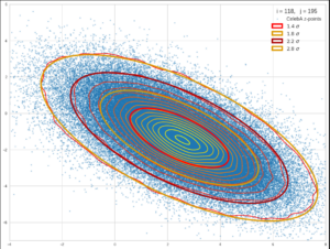
The data points correspond to vectors in the multidimensional latent space of a Convolutional AutoEncoder [CAE]. Each vector represents an image of a face after having been encoded by the encoder part of the trained CAE. The vector’s endpoints were projected onto a 2-dim coordinate plane of the basic Cartesian Coordinate System [CCS] spanning the latent space. We see that the contours of the resulting (projected) two 2-dimensional probability density are concentric ellipses whose main axes all point in the same directions. The axes of the ellipses obviously are rotated against the CCS axes. In future posts of this blog we will proof that the rotation angle of such ellipses directly depend on the correlation coefficient between underlying 1-dimensional distributions. The math of bivariate and multivariate distributions is also of further importance in ML-applications applied to data of industrial processes.

Formal definition of the covariance of two random variables X and Y

Let us abbreviate the expectation values of the random variables X and Y as E[X] and E[Y], respectively. Then the formal definition of the covariance of X and Y is:

\[ Cov(X, Y) \,=\, E \left[ \, \left( X – E \left[ X \right] \right) \left( Y – E\left[ Y \right] \right) \, \right] \, = \, E \left[ XY \right] \,-\, E \left[ X \right] E \left[ Y \right] \,. \tag{1} \]

XY is a combined two-dimensional distribution, which is defined by a probability density function g(x,y) resulting from a probability g_x(x) of X assuming x and a conditional probability c_y(y|x) of Y assuming y under the condition of X = x :

\[ g(x,y) = c_y(y|x) * g_x(x) \,=\, c_x(x|y) * g_y(y) \,. \]

The second part giving rise to symmetry arguments. Then in general we have

\[ E\left[ X Y \right] \,=\, \int_{- \infty}^{\infty} \int_{- \infty}^{\infty} xy \, g(x, y) \, dxdy \, .\tag{2} \]

The correlation coefficient ρ for the two random distributions is defined by looking at the standardized distributions :

\[ X_n \, =\, { X – E[X] \over \sigma_x}, \quad X_n \, =\, { X – E[X] \over \sigma_x} \, \Rightarrow \, \rho_{X,Y} \,=\, Cov(X_n, Y_n) \,, \]

which after some elementary consideration gives us

\[ \rho_{X,Y} \,=\, {Cov(X, Y) \over \sqrt{ Var[X] } \sqrt{Var[Y] } } \,=\, {Cov(X, Y) \over \sigma_x \ \sigma_y } \,. \tag{3} \]

To simplify the following steps we choose a 2-dimensional Cartesian coordinate system [CCS] centered such that E[X] = 0 and E[Y] = 0.

\[ \mbox{centered CCS :} \quad E \left[ X \right] = E \left[ Y \right] = 0 \, \Rightarrow \, Cov(X, Y) \,=\, E \left[ X Y \right] \,. \tag{4} \]

In the case of a centered “Bivariate Normal Distribution” [BVD] we call the respective probability function g_2c(x,y) (see a previous post) . A centered BVD can always be achieved by moving the origin of the CCS appropriately. Using this pdf we find that we have to solve the following integral:

\[ Cov(X,Y) \,=\, E\left[ X Y \right] \,=\, \int_{- \infty}^{\infty} \int_{- \infty}^{\infty} xy \, g_{2c}(x, y) \, dx\,dy \,. \tag{5} \]

Useful integral formulas

We need formulas for two integrals :

\[ \int_{- \infty}^{\infty} y * \operatorname{exp} \left( – A \left( y \,-\, C \right)^2 \right) \, dy \,=\, C\,\sqrt{ {\pi \over A}} \,, \tag{6} \]

\[ \int_{- \infty}^{\infty} y^2 * \operatorname{exp} \left( – a y^2 \right) \,dy \,=\, {1 \over 2} \sqrt{ {\pi \over a^3} \,} \,. \tag{7} \]

Performing the integration

Assumptions on the marginal distributions X and Y (having variances σ_x² and σ_y²) of a BVD and the application of symmetry arguments plus normalization conditions have revealed the general form of g₂(x,y). See the preceding post in this blog. In our centered CCS the pdf of the (centered) BVD is given by

\[ g_{2c}(x, y) \,=\, {1 \over 2 \pi \, \sigma_x \, \sigma_y } {1 \over { \sqrt{\, 1\,-\, \rho^2}} } \operatorname{exp} \left( – {1\over2} {1 \over 1\,-\, \rho^2 } \left[ {x^2 \over \sigma_x^2} \,-\, 2 \rho \, {x \over \sigma_x} {y \over \sigma_y} \,+\, {y^2 \over \sigma_y^2} \, \right] \right) \,. \tag{8} \]

ρ is a parameter and constant in this formula. We know already that it might have to to with the correlation of the random variables X and Y. To prove this analytically we now perform the required integration to get an analytical expression for the covariance.

\[ Cov(X, Y) \,=\, \\[10pt] {1 \over 2 \pi \, \sigma_x \, \sigma_y } {1 \over { \sqrt{\, 1\,-\, \rho^2}} } \int_{- \infty}^{\infty} \int_{- \infty}^{\infty} x*y* \operatorname{exp} \left( – {1\over2} {1 \over 1\,-\, \rho^2 } \left[ {x^2 \over \sigma_x^2} \,-\, 2 \rho \, {x \over \sigma_x} {y \over \sigma_y} \,+\, {y^2 \over \sigma_y^2} \, \right] \right) \, dx\,dy \,. \tag{9} \]

The trick to solve the integral over y is to complete the expression in the exponential such that we get a full square. First we redefine some variables

\[ y_{\sigma} = {y \over \sigma_y}, \quad x_{\sigma} = {x \over \sigma_x}, \quad C_x \,=\, \rho * x_\sigma, \quad A = {1 \over 2}{1 \over 1- \rho^2} \,. \tag{10} \]

The term in the exponential can now be rewritten as

\[ – {1\over2} {1 \over 1\,-\, \rho^2 } \left[ {x^2 \over \sigma_x^2} \,-\, 2 \rho \, {x \over \sigma_x} {y \over \sigma_y} \,+\, {y^2 \over \sigma_y^2} \, \right] \,=\, \left(y_\sigma – \ C_x \right)^2 \,+\, \left(1 – \rho^2 \right) x_\sigma^2 \,. \tag{11} \]

This gives us

\[ Cov(X,Y) = \\[10pt] {1 \over 2 \pi } {\sigma_x \sigma_y \over { \sqrt{\, 1\,-\, \rho^2}} } \int_{- \infty}^{\infty} \,x_\sigma * \operatorname{exp} \left(-A (1 – \rho^2\right) x_\sigma^2 \left[ \int_{- \infty}^{\infty} \,y_\sigma * \operatorname{exp} \left( -A (y_\sigma -C_x )^2 \right) dy_\sigma \right] \, dx_\sigma \,. \tag{12} \]

We solve the inner integral with the help of (6) to get:

\[ Cov(X,Y) = {1 \over {\sqrt{2 \pi}} } \sigma_x \sigma_y \, \rho \, \int_{- \infty}^{\infty} \, x_\sigma^2 * \operatorname{exp} \left(- {1\over 2} x_\sigma^2 \right) \, dx_\sigma \,. \tag{13} \]

By application of (7) we arrive at

\[ Cov(X,Y) = \sigma_x \sigma_y * \rho \,. \tag{14} \]

This is the result we have hoped for.

We obviously can identify the parameter ρ appearing in the probability density function of a bivariate normal distribution as the correlation coefficient between two underlying 1-dimensional marginal normal distributions.

In the preceding post we have seen that ρ appears in the matrix Σ^-1 defining the quadratic form in the exponential. With v = (x, y)^T we have

\[ \mbox{centered CCS :} \quad g_{2c}(x, y) \,=\, {1 \over 2 \pi \, \sigma_x \, \sigma_y } {1 \over { \sqrt{\, 1\,-\, \rho^2}} } \operatorname{exp} \left( – {1\over2} \, {\pmb{v}}^T \bullet \, \pmb{\Sigma}^{-1} \bullet {\pmb{v}} \, \right) \,, \tag{15} \]

\[ \pmb{\Sigma} \,=\, \begin{pmatrix} \sigma_x^2 &\rho\, \sigma_x\sigma_y \\ \rho\, \sigma_x\sigma_y & \sigma_y^2 \end{pmatrix}, \quad \pmb{\Sigma} \bullet \pmb{\Sigma}^{-1} = \mathbf I_n \,. \tag{16} \]

The central parameter ρ is also called the Pearson correlation coefficient.

For standardized Gaussian distributions X and Y (with σ_x = σ_y= 1) we get a very simple covariance matrix completely determined by ρ alone:

\[ \pmb{\Sigma}_{st} \,=\, \begin{pmatrix}1 &\rho\, \\ \rho\, & 1 \end{pmatrix} \,. \tag{17} \]

Conclusion

One can directly derive the correlation coefficient for the 1-dimensional Gaussian distributions underlying a Bivariate Normal Distribution [BVD] by deriving the expectation value for the product xy from the centered BVD’s probability density function g_2c(x,y). The integrals over x and y have analytical solutions.

In reverse we can say that a BVD can be constructed via defining a correlation between two 1-dimensional normal distributions and using the inverse of the covariance matrix to define a quadratic form of x and y in an exponential, which after a normalization gives you the probability density function of the BVD.

We shall see in further posts that such a construction has a direct geometrical interpretation. This will later on also motivate the abstract definition of general multidimensional or Multivariate Normal Distributions and their probability density functions.

In further posts on BVDs I will derive the probability density in a more formal way, namely by a linear transformation of a random vector of two independent 1-dimensional normal Gaussian distributions. Stay tuned …